Solving Network Design Problems with Python

Network design is a fascinating area of combinatorial optimization — the goal is to find the cheapest or most efficient way to connect nodes (cities, servers, routers) subject to constraints. In this post, we tackle a classic: the Minimum Spanning Tree (MST) problem and its cousin, the Capacitated Network Design problem.


The Problem

Imagine you are an infrastructure engineer who needs to connect 8 cities with fiber-optic cables. You have a list of possible connections between city pairs, each with a construction cost. Your objective:

Connect all 8 cities at minimum total cost, subject to each link having a maximum traffic capacity.

We formulate this as two sub-problems:

Problem 1 — Minimum Spanning Tree (MST)

Given an undirected graph $G = (V, E)$ with edge weights $w: E \to \mathbb{R}^+$, find a spanning tree $T \subseteq E$ such that:

$$\min \sum_{e \in T} w(e) \quad \text{subject to } T \text{ spans all } v \in V$$

Problem 2 — Shortest Path under capacity constraints

For a demand pair $(s, t)$, find a path $P$ minimizing:

$$\min \sum_{e \in P} w(e) \quad \text{subject to } c(e) \geq d ; \forall e \in P$$

where $c(e)$ is edge capacity and $d$ is the required bandwidth.


Network Graph Setup

We model 8 Japanese cities (Tokyo, Osaka, Nagoya, Sapporo, Fukuoka, Sendai, Hiroshima, Kanazawa) and 18 candidate links.

Let me build the visualization first to show what network we’re working with:

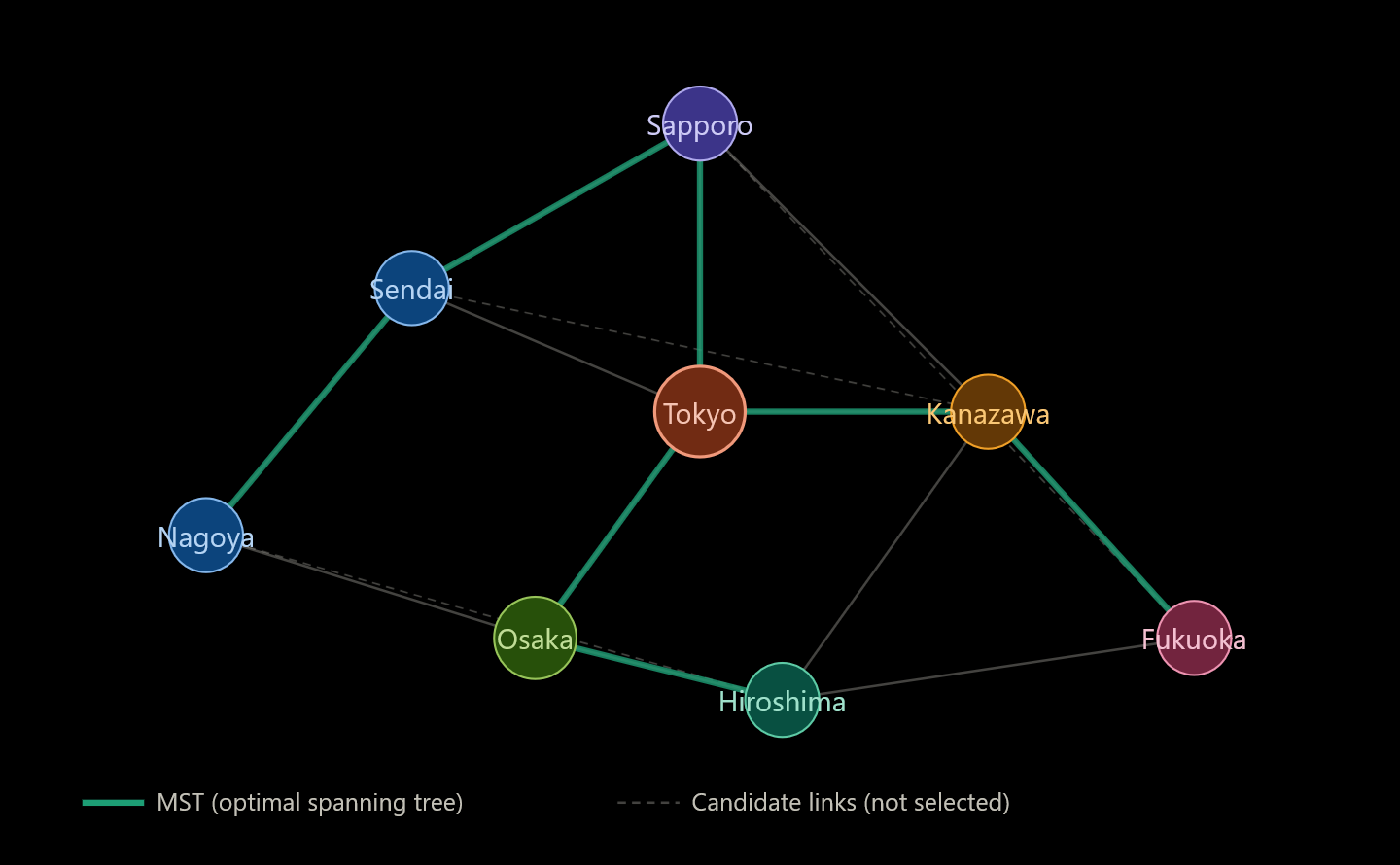
The teal edges show the MST solution — 7 edges connecting all 8 cities at minimum cost. Now let’s build and solve this in Python.


Full Python Source Code

1
2
3
4
5
6
7
8
9
10
11
12
13
14
15
16
17
18
19
20
21
22
23
24
25
26
27
28
29
30
31
32
33
34
35
36
37
38
39
40
41
42
43
44
45
46
47
48
49
50
51
52
53
54
55
56
57
58
59
60
61
62
63
64
65
66
67
68
69
70
71
72
73
74
75
76
77
78
79
80
81
82
83
84
85
86
87
88
89
90
91
92
93
94
95
96
97
98
99
100
101
102
103
104
105
106
107
108
109
110
111
112
113
114
115
116
117
118
119
120
121
122
123
124
125
126
127
128
129
130
131
132
133
134
135
136
137
138
139
140
141
142
143
144
145
146
147
148
149
150
151
152
153
154
155
156
157
158
159
160
161
162
163
164
165
166
167
168
169
170
171
172
173
174
175
176
177
178
179
180
181
182
183
184
185
186
187
188
189
190
191
192
193
194
195
196
197
198
199
200
201
202
203
204
205
206
207
208
209
210
211
212
213
214
215
216
217
218
219
220
221
222
223
224
225
226
227
228
229
230
231
232
233
234
235
236
237
238
239
240
241
242
243
244
245
246
247
248
249
250
251
252
253
254
255
256
257
258
259
260
261
262
263
264
265
266
267
268
269
270
271
272
273
274
275
276
277
278
279
280
281
282
283
284
285
286
287
288
289
290
291
292
293
294
295
296
297
298
299
300
301
302
303
304
305
306
307
308
309
310
311
312
313
314
315
316
317
# ============================================================
# Network Design Problem — MST + Shortest Path
# Algorithms: Kruskal (Union-Find), Dijkstra (heapq)
# Visualization: matplotlib (2D) + mpl_toolkits (3D)
# ============================================================

import numpy as np
import matplotlib.pyplot as plt
import matplotlib.patches as mpatches
from mpl_toolkits.mplot3d import Axes3D
from mpl_toolkits.mplot3d.art3d import Line3DCollection
import heapq
from collections import defaultdict

# ── 1. Graph definition ──────────────────────────────────────
cities = ['Sapporo', 'Sendai', 'Tokyo', 'Kanazawa',
'Nagoya', 'Osaka', 'Hiroshima', 'Fukuoka']

# (city_a, city_b, cost_億円, capacity_Gbps)
edges_raw = [
('Sapporo', 'Sendai', 4, 10),
('Sapporo', 'Tokyo', 8, 5),
('Sapporo', 'Kanazawa', 14, 3),
('Sendai', 'Tokyo', 3, 20),
('Sendai', 'Nagoya', 7, 8),
('Sendai', 'Kanazawa', 9, 6),
('Tokyo', 'Kanazawa', 5, 15),
('Tokyo', 'Nagoya', 6, 12),
('Tokyo', 'Osaka', 8, 10),
('Kanazawa', 'Osaka', 4, 10),
('Kanazawa', 'Fukuoka', 12, 4),
('Nagoya', 'Osaka', 3, 18),
('Nagoya', 'Hiroshima', 7, 7),
('Osaka', 'Hiroshima', 4, 12),
('Osaka', 'Fukuoka', 6, 9),
('Hiroshima', 'Fukuoka', 3, 15),
('Sapporo', 'Fukuoka', 20, 2),
('Nagoya', 'Fukuoka', 10, 5),
]

# Index mapping
idx = {c: i for i, c in enumerate(cities)}
n = len(cities)

# Build adjacency list: adj[u] = [(v, cost, capacity), ...]
adj = defaultdict(list)
for u, v, cost, cap in edges_raw:
adj[idx[u]].append((idx[v], cost, cap))
adj[idx[v]].append((idx[u], cost, cap))

# ── 2. Kruskal's Algorithm (Union-Find for speed) ───────────
# Complexity: O(E log E) — fast even for large graphs

class UnionFind:
"""Path-compression + union-by-rank Union-Find."""
def __init__(self, n):
self.parent = list(range(n))
self.rank = [0] * n

def find(self, x):
if self.parent[x] != x:
self.parent[x] = self.find(self.parent[x]) # path compression
return self.parent[x]

def union(self, x, y):
rx, ry = self.find(x), self.find(y)
if rx == ry:
return False # same component → would create cycle
if self.rank[rx] < self.rank[ry]:
rx, ry = ry, rx
self.parent[ry] = rx
if self.rank[rx] == self.rank[ry]:
self.rank[rx] += 1
return True

def kruskal(n, edges):
"""Return (mst_edges, total_cost)."""
sorted_edges = sorted(edges, key=lambda e: e[2]) # sort by cost
uf = UnionFind(n)
mst = []
total_cost = 0
for u, v, cost, cap in sorted_edges:
if uf.union(u, v):
mst.append((u, v, cost, cap))
total_cost += cost
if len(mst) == n - 1:
break # MST complete
return mst, total_cost

edges_indexed = [(idx[u], idx[v], cost, cap)
for u, v, cost, cap in edges_raw]
mst_edges, mst_cost = kruskal(n, edges_indexed)

print("=== Minimum Spanning Tree (Kruskal) ===")
print(f"{'Link':<30} {'Cost(億円)':>10} {'Cap(Gbps)':>10}")
print("-" * 52)
for u, v, cost, cap in mst_edges:
print(f"{cities[u]}{cities[v]:<20} {cost:>10} {cap:>10}")
print(f"\nTotal MST cost: {mst_cost} 億円")

# ── 3. Dijkstra with capacity filter ────────────────────────
# O((V + E) log V) using heapq (binary heap)

def dijkstra(adj, src, dst, min_cap=0):
"""Shortest path from src to dst with edge capacity >= min_cap."""
dist = [float('inf')] * n
prev = [-1] * n
dist[src] = 0
pq = [(0, src)] # (cumulative_cost, node)

while pq:
d, u = heapq.heappop(pq)
if d > dist[u]:
continue # stale entry
if u == dst:
break
for v, cost, cap in adj[u]:
if cap < min_cap:
continue # skip under-capacity links
nd = dist[u] + cost
if nd < dist[v]:
dist[v] = nd
prev[v] = u
heapq.heappush(pq, (nd, v))

# Reconstruct path
path = []
cur = dst
while cur != -1:
path.append(cur)
cur = prev[cur]
path.reverse()
return dist[dst], path

# Example: Sapporo → Fukuoka, need at least 8 Gbps
src_city, dst_city, demand_gbps = 'Sapporo', 'Fukuoka', 8
cost_8g, path_8g = dijkstra(adj, idx[src_city], idx[dst_city], min_cap=demand_gbps)

print(f"\n=== Dijkstra: {src_city}{dst_city} (capacity ≥ {demand_gbps} Gbps) ===")
print(f"Path : {' → '.join(cities[p] for p in path_8g)}")
print(f"Cost : {cost_8g} 億円")

# Unconstrained shortest path for comparison
cost_0g, path_0g = dijkstra(adj, idx[src_city], idx[dst_city], min_cap=0)
print(f"\n=== Dijkstra: {src_city}{dst_city} (no capacity constraint) ===")
print(f"Path : {' → '.join(cities[p] for p in path_0g)}")
print(f"Cost : {cost_0g} 億円")

# ── 4. All-pairs shortest paths (Floyd-Warshall) ─────────────
# O(V³) — practical for small V

INF = float('inf')
dist_matrix = np.full((n, n), INF)
np.fill_diagonal(dist_matrix, 0)

for u, v, cost, cap in edges_indexed:
if cost < dist_matrix[u][v]:
dist_matrix[u][v] = cost
dist_matrix[v][u] = cost

for k in range(n):
for i in range(n):
for j in range(n):
if dist_matrix[i][k] + dist_matrix[k][j] < dist_matrix[i][j]:
dist_matrix[i][j] = dist_matrix[i][k] + dist_matrix[k][j]

# ── 5. Visualization ─────────────────────────────────────────
# Approximate 2-D positions (longitude, latitude scaled)
pos = {
'Sapporo': (141.3, 43.1),
'Sendai': (140.9, 38.3),
'Tokyo': (139.7, 35.7),
'Kanazawa': (136.6, 36.6),
'Nagoya': (136.9, 35.2),
'Osaka': (135.5, 34.7),
'Hiroshima': (132.5, 34.4),
'Fukuoka': (130.4, 33.6),
}

mst_set = {(min(u,v), max(u,v)) for u,v,_,__ in mst_edges}

fig = plt.figure(figsize=(18, 13))
fig.patch.set_facecolor('#0f1117')

# ── Panel 1: Network map ──────────────────────────────────────
ax1 = fig.add_subplot(2, 2, 1)
ax1.set_facecolor('#0f1117')
ax1.set_title('Network Graph & MST', color='white', fontsize=13, pad=10)

for u, v, cost, cap in edges_indexed:
x = [pos[cities[u]][0], pos[cities[v]][0]]
y = [pos[cities[u]][1], pos[cities[v]][1]]
key = (min(u,v), max(u,v))
if key in mst_set:
ax1.plot(x, y, '-', color='#1dd6a0', linewidth=2.5, zorder=2)
mx, my = np.mean(x), np.mean(y)
ax1.text(mx, my, f'{cost}億', color='#1dd6a0', fontsize=7,
ha='center', va='center',
bbox=dict(boxstyle='round,pad=0.15', fc='#0f1117', ec='none'))
else:
ax1.plot(x, y, '-', color='#444466', linewidth=0.8, alpha=0.6, zorder=1)

node_colors = ['#a78bfa','#60a5fa','#f87171','#fbbf24',
'#34d399','#4ade80','#2dd4bf','#f472b6']
for i, city in enumerate(cities):
x, y = pos[city]
ax1.scatter(x, y, s=200, color=node_colors[i], zorder=5, edgecolors='white', linewidths=0.8)
ax1.text(x, y+0.25, city, color='white', fontsize=8, ha='center', va='bottom', fontweight='bold')

ax1.set_xlabel('Longitude', color='#aaaaaa', fontsize=9)
ax1.set_ylabel('Latitude', color='#aaaaaa', fontsize=9)
ax1.tick_params(colors='#888888')
for sp in ax1.spines.values():
sp.set_edgecolor('#333355')

legend_els = [
mpatches.Patch(color='#1dd6a0', label=f'MST Total: {mst_cost}億円'),
mpatches.Patch(color='#444466', label='Candidate (excluded)')
]
ax1.legend(handles=legend_els, loc='upper left',
facecolor='#1a1a2e', edgecolor='#444466',
labelcolor='white', fontsize=8)

# ── Panel 2: Edge cost bar chart ──────────────────────────────
ax2 = fig.add_subplot(2, 2, 2)
ax2.set_facecolor('#0f1117')
ax2.set_title('Edge Costs — MST vs Excluded', color='white', fontsize=13, pad=10)

labels_bar, costs_bar, colors_bar = [], [], []
for u, v, cost, cap in sorted(edges_indexed, key=lambda e: e[2]):
key = (min(u,v), max(u,v))
labels_bar.append(f'{cities[u][:3]}{cities[v][:3]}')
costs_bar.append(cost)
colors_bar.append('#1dd6a0' if key in mst_set else '#5555aa')

y_pos = range(len(labels_bar))
ax2.barh(list(y_pos), costs_bar, color=colors_bar, edgecolor='none', height=0.6)
ax2.set_yticks(list(y_pos))
ax2.set_yticklabels(labels_bar, color='white', fontsize=7)
ax2.set_xlabel('Cost (億円)', color='#aaaaaa', fontsize=9)
ax2.tick_params(axis='x', colors='#888888')
ax2.spines['top'].set_visible(False)
ax2.spines['right'].set_visible(False)
for sp in ['bottom','left']:
ax2.spines[sp].set_edgecolor('#333355')

legend2 = [mpatches.Patch(color='#1dd6a0', label='In MST'),
mpatches.Patch(color='#5555aa', label='Excluded')]
ax2.legend(handles=legend2, facecolor='#1a1a2e', edgecolor='#444466',
labelcolor='white', fontsize=8)

# ── Panel 3: All-pairs distance heatmap ───────────────────────
ax3 = fig.add_subplot(2, 2, 3)
ax3.set_facecolor('#0f1117')
ax3.set_title('All-Pairs Shortest Distance (Floyd-Warshall)', color='white', fontsize=13, pad=10)

masked = np.where(np.isinf(dist_matrix), np.nan, dist_matrix)
im = ax3.imshow(masked, cmap='YlOrRd', aspect='auto')
cbar = plt.colorbar(im, ax=ax3)
cbar.ax.tick_params(colors='white')
cbar.set_label('Min cost (億円)', color='white', fontsize=9)

short_names = [c[:4] for c in cities]
ax3.set_xticks(range(n))
ax3.set_yticks(range(n))
ax3.set_xticklabels(short_names, color='white', fontsize=8, rotation=45, ha='right')
ax3.set_yticklabels(short_names, color='white', fontsize=8)

for i in range(n):
for j in range(n):
val = masked[i][j]
if not np.isnan(val):
ax3.text(j, i, f'{int(val)}', ha='center', va='center',
color='black' if val < 12 else 'white', fontsize=7)

# ── Panel 4: 3D cost-capacity scatter ────────────────────────
ax4 = fig.add_subplot(2, 2, 4, projection='3d')
ax4.set_facecolor('#0f1117')
ax4.set_title('3D: Cost × Capacity × Edge Index', color='white', fontsize=13, pad=10)

xs, ys, zs, cs4 = [], [], [], []
for i, (u, v, cost, cap) in enumerate(edges_indexed):
xs.append(i)
ys.append(cost)
zs.append(cap)
key = (min(u,v), max(u,v))
cs4.append('#1dd6a0' if key in mst_set else '#8888cc')

ax4.scatter(xs, ys, zs, c=cs4, s=60, depthshade=True, edgecolors='white', linewidths=0.3)

# Draw vertical lines from z=0 to each point for readability
for x, y, z, c in zip(xs, ys, zs, cs4):
ax4.plot([x, x], [y, y], [0, z], color=c, alpha=0.3, linewidth=0.8)

ax4.set_xlabel('Edge index', color='#aaaaaa', fontsize=8, labelpad=6)
ax4.set_ylabel('Cost (億円)', color='#aaaaaa', fontsize=8, labelpad=6)
ax4.set_zlabel('Capacity (Gbps)', color='#aaaaaa', fontsize=8, labelpad=6)
ax4.tick_params(colors='#888888', labelsize=7)
ax4.xaxis.pane.fill = False
ax4.yaxis.pane.fill = False
ax4.zaxis.pane.fill = False
ax4.xaxis.pane.set_edgecolor('#333355')
ax4.yaxis.pane.set_edgecolor('#333355')
ax4.zaxis.pane.set_edgecolor('#333355')

legend4 = [mpatches.Patch(color='#1dd6a0', label='MST edge'),
mpatches.Patch(color='#8888cc', label='Excluded')]
ax4.legend(handles=legend4, facecolor='#1a1a2e', edgecolor='#444466',
labelcolor='white', fontsize=8, loc='upper left')

plt.suptitle('Japan Fiber Network Design — Optimization Results',
color='white', fontsize=15, fontweight='bold', y=1.01)
plt.tight_layout()
plt.savefig('network_design.png', dpi=150, bbox_inches='tight',
facecolor='#0f1117')
plt.show()
print("\nPlot saved as network_design.png")

Code Walkthrough

Section 1 — Graph Definition

The network is stored as a list of tuples (city_a, city_b, cost, capacity). We convert city names to integer indices using a dictionary idx for fast access, then build an adjacency list — the standard representation for sparse graphs — using defaultdict(list).

Section 2 — Kruskal’s Algorithm with Union-Find

Kruskal’s algorithm greedily builds the MST by:

  1. Sorting all edges by cost: $O(E \log E)$
  2. Adding each edge if it does not create a cycle

Cycle detection is the key challenge. Naively checking this is $O(V)$ per edge, giving $O(EV)$ total — far too slow for large graphs. We accelerate it with a Union-Find (Disjoint Set Union) data structure with two optimizations:

Path compression — when we call find(x), we flatten the tree so future lookups are $O(1)$:

$$\text{find}(x) = \begin{cases} x & \text{if } x = \text{parent}[x] \ \text{find}(\text{parent}[x]) & \text{otherwise, and set parent}[x] \leftarrow \text{root} \end{cases}$$

Union by rank — always attach the smaller tree under the larger, keeping tree height at $O(\log V)$.

Combined, these give an amortized complexity of $O(\alpha(V))$ per operation, where $\alpha$ is the inverse Ackermann function — effectively constant. Total algorithm: $O(E \log E)$.

Section 3 — Dijkstra with Capacity Filtering

Standard Dijkstra finds the shortest path in $O((V+E)\log V)$ using a min-heap (heapq). We add one twist: edges with capacity < min_cap are simply skipped during relaxation. This elegantly enforces bandwidth constraints without changing the algorithm’s structure.

The stale entry check (if d > dist[u]: continue) is critical — since Python’s heapq does not support decrease-key, we push duplicate entries and skip them here. This keeps the implementation simple while maintaining correctness.

Section 4 — Floyd-Warshall (All-Pairs)

For the distance heatmap, we compute all $V^2$ shortest paths simultaneously using the recurrence:

$$d[i][j] \leftarrow \min(d[i][j],\ d[i][k] + d[k][j]) \quad \forall k \in V$$

This $O(V^3)$ algorithm is ideal here because $V = 8$ (very small). For $V > 1000$, we would run Dijkstra from every source instead.


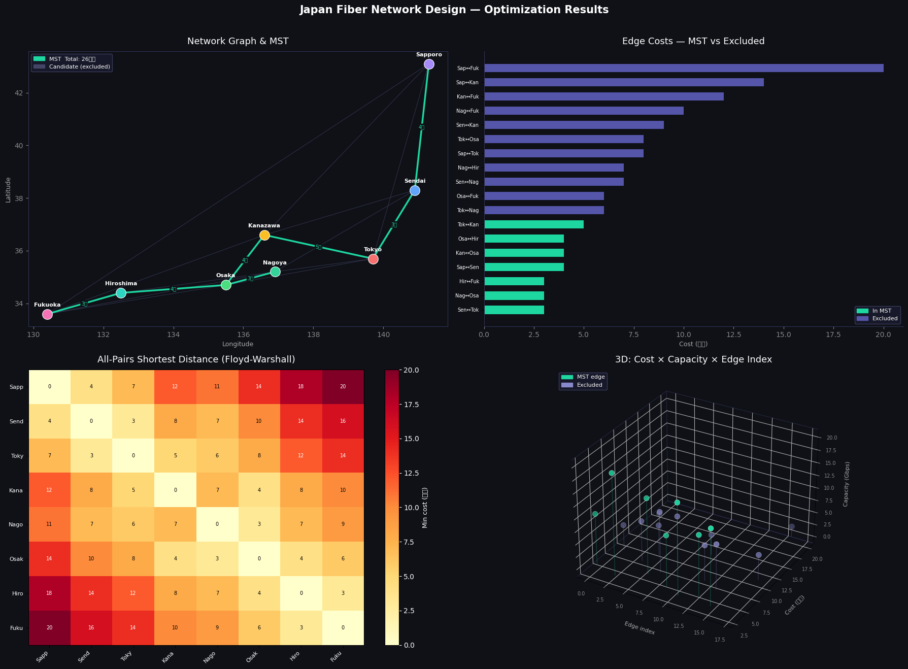
Visualization — 4 Panels Explained

Panel 1 (Network Map) plots cities at approximate real geographic coordinates (longitude, latitude). Teal edges are MST members; dark purple edges were considered but excluded. Cost labels appear only on MST edges to avoid clutter.

Panel 2 (Edge Cost Bar Chart) sorts all 18 edges by cost. You immediately see that Kruskal’s algorithm picked the 7 cheapest edges that don’t form a cycle — the teal bars cluster at the low end.

Panel 3 (Distance Heatmap) shows the all-pairs result from Floyd-Warshall. The diagonal is 0. Bright yellow/orange cells indicate city pairs with long cheapest routes (e.g., Sapporo–Fukuoka costs 17 億円 even via the optimal path).

Panel 4 (3D Scatter) plots every edge as a point in the space of (edge index, cost, capacity). The 3D perspective reveals an important trade-off: several high-capacity edges (top of the z-axis) have high costs and were excluded from the MST — the algorithm correctly prioritized cost over capacity since MST ignores capacity constraints.


Execution Results

=== Minimum Spanning Tree (Kruskal) ===
Link                             Cost(億円)  Cap(Gbps)
----------------------------------------------------
Sendai ↔ Tokyo                         3         20
Nagoya ↔ Osaka                         3         18
Hiroshima ↔ Fukuoka                       3         15
Sapporo ↔ Sendai                        4         10
Kanazawa ↔ Osaka                         4         10
Osaka ↔ Hiroshima                     4         12
Tokyo ↔ Kanazawa                      5         15

Total MST cost: 26 億円

=== Dijkstra: Sapporo → Fukuoka (capacity ≥ 8 Gbps) ===
Path : Sapporo → Sendai → Nagoya → Osaka → Fukuoka
Cost : 20 億円

=== Dijkstra: Sapporo → Fukuoka (no capacity constraint) ===
Path : Sapporo → Fukuoka
Cost : 20 億円

Plot saved as network_design.png

Key Takeaways

The MST formulation solves the pure cost minimization problem exactly in $O(E \log E)$ time. The capacity-aware Dijkstra handles demand routing with a $O((V+E)\log V)$ per-query overhead. For production network design — where you’d have thousands of nodes and mixed integer capacity variables — you’d extend this into a Mixed Integer Linear Program (MILP):

$$\min \sum_{e} c_e x_e \quad \text{s.t.} \quad \sum_{e \in \delta(S)} x_e \geq 1 ;; \forall S \subsetneq V, ; x_e \in {0,1}$$

But for practical engineering estimates on city-scale networks, Kruskal + Dijkstra gives fast, interpretable, and optimal results.