๐Ÿญ Production Lot Size Problem with Integer Constraints

๐Ÿ“Œ Problem Overview

The Production Lot Size Problem (also known as the Capacitated Lot Sizing Problem, CLSP) asks: How many units of each product should we produce in each period to minimize total costs, while satisfying demand and not exceeding production capacity?

When lot sizes must be integers (you canโ€™t produce half a unit), this becomes a Mixed-Integer Programming (MIP) problem โ€” significantly harder than its continuous cousin.


๐Ÿงฎ Mathematical Formulation

Sets & Indices:

  • $i \in {1, \ldots, N}$: products
  • $t \in {1, \ldots, T}$: time periods

Decision Variables:

  • $x_{it} \in \mathbb{Z}_{\geq 0}$: production quantity of product $i$ in period $t$ (integer)
  • $y_{it} \in {0, 1}$: setup indicator (1 if product $i$ is produced in period $t$)
  • $s_{it} \geq 0$: inventory of product $i$ at end of period $t$

Parameters:

  • $d_{it}$: demand for product $i$ in period $t$
  • $p_i$: unit production cost for product $i$
  • $h_i$: unit holding cost per period for product $i$
  • $f_i$: fixed setup cost for product $i$
  • $c_t$: capacity available in period $t$
  • $a_i$: capacity consumed per unit of product $i$
  • $M$: big-M constant

Objective โ€” Minimize total cost:

$$\min \sum_{i=1}^{N} \sum_{t=1}^{T} \left( p_i x_{it} + h_i s_{it} + f_i y_{it} \right)$$

Subject to:

Inventory balance:
$$s_{i,t-1} + x_{it} - s_{it} = d_{it} \quad \forall i, t$$

Capacity constraint:
$$\sum_{i=1}^{N} a_i x_{it} \leq c_t \quad \forall t$$

Setup linkage (Big-M):
$$x_{it} \leq M \cdot y_{it} \quad \forall i, t$$

Integrality & non-negativity:
$$x_{it} \in \mathbb{Z}{\geq 0}, \quad y{it} \in {0,1}, \quad s_{it} \geq 0$$


๐Ÿ—๏ธ Concrete Example

We have 3 products over 6 periods.

Product $p_i$ (prod cost) $h_i$ (hold cost) $f_i$ (setup cost) $a_i$ (capacity/unit)
A 10 2 50 3
B 15 3 80 4
C 12 2.5 60 2

Demand $d_{it}$:

Period Product A Product B Product C
1 20 15 25
2 30 20 20
3 25 25 30
4 20 15 25
5 35 30 20
6 25 20 30

Capacity per period: $c_t = 300$ for all $t$


๐Ÿ’ป Python Source Code

1
2
3
4
5
6
7
8
9
10
11
12
13
14
15
16
17
18
19
20
21
22
23
24
25
26
27
28
29
30
31
32
33
34
35
36
37
38
39
40
41
42
43
44
45
46
47
48
49
50
51
52
53
54
55
56
57
58
59
60
61
62
63
64
65
66
67
68
69
70
71
72
73
74
75
76
77
78
79
80
81
82
83
84
85
86
87
88
89
90
91
92
93
94
95
96
97
98
99
100
101
102
103
104
105
106
107
108
109
110
111
112
113
114
115
116
117
118
119
120
121
122
123
124
125
126
127
128
129
130
131
132
133
134
135
136
137
138
139
140
141
142
143
144
145
146
147
148
149
150
151
152
153
154
155
156
157
158
159
160
161
162
163
164
165
166
167
168
169
170
171
172
173
174
175
176
177
178
179
180
181
182
183
184
185
186
187
188
189
190
191
192
193
194
195
196
197
198
199
200
201
202
203
204
205
206
207
208
209
210
211
212
213
214
215
216
217
218
219
220
221
222
223
224
225
226
227
228
229
230
231
232
233
234
235
236
237
238
239
240
241
242
243
244
245
246
247
248
249
250
251
252
253
254
255
256
257
258
259
260
261
262
263
264
265
266
267
268
269
270
271
272
273
274
275
276
277
278
279
280
281
282
283
284
285
286
287
288
289
290
291
292
293
294
295
296
297
298
299
300
301
302
# ============================================================
# Production Lot Size Problem with Integer Constraints
# Solver: PuLP (CBC MIP solver)
# ============================================================

import numpy as np
import matplotlib.pyplot as plt
import matplotlib.gridspec as gridspec
from mpl_toolkits.mplot3d import Axes3D
import pulp
import warnings
warnings.filterwarnings('ignore')

# โ”€โ”€ 1. Problem Data โ”€โ”€โ”€โ”€โ”€โ”€โ”€โ”€โ”€โ”€โ”€โ”€โ”€โ”€โ”€โ”€โ”€โ”€โ”€โ”€โ”€โ”€โ”€โ”€โ”€โ”€โ”€โ”€โ”€โ”€โ”€โ”€โ”€โ”€โ”€โ”€โ”€โ”€โ”€โ”€โ”€
N = 3 # number of products
T = 6 # number of periods

products = ['Product A', 'Product B', 'Product C']
periods = list(range(1, T + 1))

# Unit production cost
p = [10, 15, 12]

# Unit holding cost per period
h = [2, 3, 2.5]

# Fixed setup cost
f = [50, 80, 60]

# Capacity consumption per unit
a = [3, 4, 2]

# Capacity per period
C = [300] * T

# Demand d[i][t] (0-indexed)
d = np.array([
[20, 30, 25, 20, 35, 25], # Product A
[15, 20, 25, 15, 30, 20], # Product B
[25, 20, 30, 25, 20, 30], # Product C
])

# Big-M: safe upper bound on production per product per period
M_val = int(np.sum(d, axis=1).max() * T)

# โ”€โ”€ 2. Build MIP Model โ”€โ”€โ”€โ”€โ”€โ”€โ”€โ”€โ”€โ”€โ”€โ”€โ”€โ”€โ”€โ”€โ”€โ”€โ”€โ”€โ”€โ”€โ”€โ”€โ”€โ”€โ”€โ”€โ”€โ”€โ”€โ”€โ”€โ”€โ”€โ”€โ”€โ”€โ”€
model = pulp.LpProblem("Lot_Sizing_Integer", pulp.LpMinimize)

# Decision variables
x = [[pulp.LpVariable(f"x_{i}_{t}", lowBound=0, cat='Integer')
for t in range(T)] for i in range(N)]

y = [[pulp.LpVariable(f"y_{i}_{t}", cat='Binary')
for t in range(T)] for i in range(N)]

s = [[pulp.LpVariable(f"s_{i}_{t}", lowBound=0, cat='Continuous')
for t in range(T)] for i in range(N)]

# Objective function
model += pulp.lpSum(
p[i] * x[i][t] + h[i] * s[i][t] + f[i] * y[i][t]
for i in range(N) for t in range(T)
), "Total_Cost"

# โ”€โ”€ 3. Constraints โ”€โ”€โ”€โ”€โ”€โ”€โ”€โ”€โ”€โ”€โ”€โ”€โ”€โ”€โ”€โ”€โ”€โ”€โ”€โ”€โ”€โ”€โ”€โ”€โ”€โ”€โ”€โ”€โ”€โ”€โ”€โ”€โ”€โ”€โ”€โ”€โ”€โ”€โ”€โ”€โ”€โ”€โ”€
for i in range(N):
for t in range(T):
# Inventory balance
prev_s = s[i][t-1] if t > 0 else 0
model += prev_s + x[i][t] - s[i][t] == d[i][t], \
f"InvBalance_{i}_{t}"

# Setup linkage (Big-M)
model += x[i][t] <= M_val * y[i][t], \
f"Setup_{i}_{t}"

for t in range(T):
# Capacity constraint
model += pulp.lpSum(a[i] * x[i][t] for i in range(N)) <= C[t], \
f"Capacity_{t}"

# โ”€โ”€ 4. Solve โ”€โ”€โ”€โ”€โ”€โ”€โ”€โ”€โ”€โ”€โ”€โ”€โ”€โ”€โ”€โ”€โ”€โ”€โ”€โ”€โ”€โ”€โ”€โ”€โ”€โ”€โ”€โ”€โ”€โ”€โ”€โ”€โ”€โ”€โ”€โ”€โ”€โ”€โ”€โ”€โ”€โ”€โ”€โ”€โ”€โ”€โ”€โ”€โ”€
solver = pulp.PULP_CBC_CMD(msg=0, timeLimit=120)
status = model.solve(solver)

print("=" * 55)
print(f" Solver Status : {pulp.LpStatus[model.status]}")
print(f" Total Cost : {pulp.value(model.objective):,.2f}")
print("=" * 55)

# โ”€โ”€ 5. Extract Results โ”€โ”€โ”€โ”€โ”€โ”€โ”€โ”€โ”€โ”€โ”€โ”€โ”€โ”€โ”€โ”€โ”€โ”€โ”€โ”€โ”€โ”€โ”€โ”€โ”€โ”€โ”€โ”€โ”€โ”€โ”€โ”€โ”€โ”€โ”€โ”€โ”€โ”€โ”€
x_val = np.array([[pulp.value(x[i][t]) for t in range(T)]
for i in range(N)])
y_val = np.array([[pulp.value(y[i][t]) for t in range(T)]
for i in range(N)])
s_val = np.array([[pulp.value(s[i][t]) for t in range(T)]
for i in range(N)])

# Compute cost components
prod_cost = np.array([[p[i] * x_val[i][t] for t in range(T)]
for i in range(N)])
hold_cost = np.array([[h[i] * s_val[i][t] for t in range(T)]
for i in range(N)])
setup_cost = np.array([[f[i] * y_val[i][t] for t in range(T)]
for i in range(N)])

cap_used = np.array([sum(a[i] * x_val[i][t] for i in range(N))
for t in range(T)])

# โ”€โ”€ 6. Print Detail Table โ”€โ”€โ”€โ”€โ”€โ”€โ”€โ”€โ”€โ”€โ”€โ”€โ”€โ”€โ”€โ”€โ”€โ”€โ”€โ”€โ”€โ”€โ”€โ”€โ”€โ”€โ”€โ”€โ”€โ”€โ”€โ”€โ”€โ”€โ”€โ”€
print("\nโ”€โ”€ Production Plan (x_it) โ”€โ”€")
header = "Product " + "".join([f" P{t+1}" for t in range(T)])
print(header)
for i in range(N):
row = f"{products[i]:<12} " + \
"".join([f"{int(x_val[i][t]):>5}" for t in range(T)])
print(row)

print("\nโ”€โ”€ Setup Decisions (y_it) โ”€โ”€")
print(header)
for i in range(N):
row = f"{products[i]:<12} " + \
"".join([f"{int(y_val[i][t]):>5}" for t in range(T)])
print(row)

print("\nโ”€โ”€ End Inventory (s_it) โ”€โ”€")
print(header)
for i in range(N):
row = f"{products[i]:<12} " + \
"".join([f"{s_val[i][t]:>5.0f}" for t in range(T)])
print(row)

print("\nโ”€โ”€ Capacity Used / Available โ”€โ”€")
for t in range(T):
util = cap_used[t] / C[t] * 100
print(f" Period {t+1}: {cap_used[t]:>6.0f} / {C[t]} "
f"({util:.1f}% utilization)")

# โ”€โ”€ 7. Visualization โ”€โ”€โ”€โ”€โ”€โ”€โ”€โ”€โ”€โ”€โ”€โ”€โ”€โ”€โ”€โ”€โ”€โ”€โ”€โ”€โ”€โ”€โ”€โ”€โ”€โ”€โ”€โ”€โ”€โ”€โ”€โ”€โ”€โ”€โ”€โ”€โ”€โ”€โ”€โ”€โ”€
colors = ['#2196F3', '#FF5722', '#4CAF50']
period_labels = [f"P{t+1}" for t in range(T)]

fig = plt.figure(figsize=(20, 22))
fig.patch.set_facecolor('#0d1117')
gs = gridspec.GridSpec(3, 2, figure=fig,
hspace=0.45, wspace=0.35)

title_kw = dict(color='white', fontsize=13, fontweight='bold', pad=10)
label_kw = dict(color='#aaaaaa', fontsize=10)
tick_kw = dict(colors='#888888', labelsize=9)

# โ”€โ”€ Plot 1: Production quantities (grouped bar) โ”€โ”€โ”€โ”€โ”€โ”€โ”€โ”€โ”€โ”€โ”€โ”€โ”€โ”€
ax1 = fig.add_subplot(gs[0, 0])
ax1.set_facecolor('#161b22')
x_pos = np.arange(T)
bw = 0.25
for i in range(N):
ax1.bar(x_pos + i * bw, x_val[i], bw,
label=products[i], color=colors[i], alpha=0.85,
edgecolor='white', linewidth=0.4)
# demand line
ax1.plot(x_pos + i * bw + bw / 2, d[i],
'o--', color=colors[i], alpha=0.5,
markersize=4, linewidth=1)
ax1.set_title("Production Quantities vs Demand", **title_kw)
ax1.set_xlabel("Period", **label_kw)
ax1.set_ylabel("Units", **label_kw)
ax1.set_xticks(x_pos + bw)
ax1.set_xticklabels(period_labels)
ax1.tick_params(axis='both', **tick_kw)
ax1.legend(fontsize=9, labelcolor='white',
facecolor='#1f2937', edgecolor='#374151')
ax1.spines[['top','right']].set_visible(False)
for sp in ['bottom','left']:
ax1.spines[sp].set_color('#374151')

# โ”€โ”€ Plot 2: Inventory levels โ”€โ”€โ”€โ”€โ”€โ”€โ”€โ”€โ”€โ”€โ”€โ”€โ”€โ”€โ”€โ”€โ”€โ”€โ”€โ”€โ”€โ”€โ”€โ”€โ”€โ”€โ”€โ”€โ”€โ”€โ”€โ”€โ”€
ax2 = fig.add_subplot(gs[0, 1])
ax2.set_facecolor('#161b22')
for i in range(N):
ax2.plot(periods, s_val[i], 'o-',
color=colors[i], label=products[i],
linewidth=2, markersize=6)
ax2.fill_between(periods, s_val[i], alpha=0.15, color=colors[i])
ax2.set_title("Ending Inventory Levels", **title_kw)
ax2.set_xlabel("Period", **label_kw)
ax2.set_ylabel("Units in Stock", **label_kw)
ax2.tick_params(axis='both', **tick_kw)
ax2.legend(fontsize=9, labelcolor='white',
facecolor='#1f2937', edgecolor='#374151')
ax2.spines[['top','right']].set_visible(False)
for sp in ['bottom','left']:
ax2.spines[sp].set_color('#374151')

# โ”€โ”€ Plot 3: Cost breakdown (stacked bar per period) โ”€โ”€โ”€โ”€โ”€โ”€โ”€โ”€โ”€โ”€
ax3 = fig.add_subplot(gs[1, 0])
ax3.set_facecolor('#161b22')
total_prod = prod_cost.sum(axis=0)
total_hold = hold_cost.sum(axis=0)
total_setup = setup_cost.sum(axis=0)
ax3.bar(period_labels, total_prod,
label='Production', color='#3b82f6', alpha=0.9)
ax3.bar(period_labels, total_hold, bottom=total_prod,
label='Holding', color='#f59e0b', alpha=0.9)
ax3.bar(period_labels, total_setup,
bottom=total_prod + total_hold,
label='Setup', color='#ef4444', alpha=0.9)
ax3.set_title("Cost Breakdown by Period", **title_kw)
ax3.set_xlabel("Period", **label_kw)
ax3.set_ylabel("Cost ($)", **label_kw)
ax3.tick_params(axis='both', **tick_kw)
ax3.legend(fontsize=9, labelcolor='white',
facecolor='#1f2937', edgecolor='#374151')
ax3.spines[['top','right']].set_visible(False)
for sp in ['bottom','left']:
ax3.spines[sp].set_color('#374151')

# โ”€โ”€ Plot 4: Capacity utilization โ”€โ”€โ”€โ”€โ”€โ”€โ”€โ”€โ”€โ”€โ”€โ”€โ”€โ”€โ”€โ”€โ”€โ”€โ”€โ”€โ”€โ”€โ”€โ”€โ”€โ”€โ”€โ”€โ”€
ax4 = fig.add_subplot(gs[1, 1])
ax4.set_facecolor('#161b22')
util_pct = cap_used / np.array(C) * 100
bar_colors = ['#ef4444' if u > 90 else '#22c55e' for u in util_pct]
ax4.bar(period_labels, util_pct, color=bar_colors,
alpha=0.85, edgecolor='white', linewidth=0.4)
ax4.axhline(100, color='#ef4444', linestyle='--',
linewidth=1.5, label='Capacity limit')
ax4.axhline(80, color='#f59e0b', linestyle=':',
linewidth=1, label='80% threshold')
ax4.set_title("Capacity Utilization (%)", **title_kw)
ax4.set_xlabel("Period", **label_kw)
ax4.set_ylabel("Utilization (%)", **label_kw)
ax4.set_ylim(0, 110)
ax4.tick_params(axis='both', **tick_kw)
ax4.legend(fontsize=9, labelcolor='white',
facecolor='#1f2937', edgecolor='#374151')
ax4.spines[['top','right']].set_visible(False)
for sp in ['bottom','left']:
ax4.spines[sp].set_color('#374151')

# โ”€โ”€ Plot 5: 3D โ€” Production x_it as surface/bar3d โ”€โ”€โ”€โ”€โ”€โ”€โ”€โ”€โ”€โ”€โ”€โ”€
ax5 = fig.add_subplot(gs[2, 0], projection='3d')
ax5.set_facecolor('#161b22')
fig.patch.set_alpha(1)
_x = np.arange(N)
_t = np.arange(T)
_xx, _tt = np.meshgrid(_x, _t)
xx_flat = _xx.ravel()
tt_flat = _tt.ravel()
zz_flat = x_val[xx_flat, tt_flat]
bar_c = [colors[i] for i in xx_flat]

ax5.bar3d(xx_flat - 0.3, tt_flat - 0.3, np.zeros_like(zz_flat),
0.6, 0.6, zz_flat,
color=bar_c, alpha=0.75, shade=True)
ax5.set_title("3D: Production Quantities\n(Product ร— Period)",
color='white', fontsize=12, fontweight='bold')
ax5.set_xlabel("Product", color='#aaaaaa', labelpad=8)
ax5.set_ylabel("Period", color='#aaaaaa', labelpad=8)
ax5.set_zlabel("Units", color='#aaaaaa', labelpad=8)
ax5.set_xticks([0, 1, 2])
ax5.set_xticklabels(['A', 'B', 'C'], color='#888888')
ax5.set_yticks(range(T))
ax5.set_yticklabels([f"P{t+1}" for t in range(T)], color='#888888')
ax5.tick_params(colors='#888888')
ax5.xaxis.pane.fill = False
ax5.yaxis.pane.fill = False
ax5.zaxis.pane.fill = False
ax5.grid(color='#374151', linestyle='--', alpha=0.3)

# โ”€โ”€ Plot 6: 3D โ€” Cost surface โ”€โ”€โ”€โ”€โ”€โ”€โ”€โ”€โ”€โ”€โ”€โ”€โ”€โ”€โ”€โ”€โ”€โ”€โ”€โ”€โ”€โ”€โ”€โ”€โ”€โ”€โ”€โ”€โ”€โ”€โ”€โ”€
ax6 = fig.add_subplot(gs[2, 1], projection='3d')
ax6.set_facecolor('#161b22')
total_cost_it = prod_cost + hold_cost + setup_cost # shape (N, T)
X6, T6 = np.meshgrid(np.arange(T), np.arange(N))
ax6.plot_surface(X6, T6, total_cost_it,
cmap='plasma', alpha=0.85,
edgecolor='none')
ax6.set_title("3D: Cost Surface\n(Product ร— Period)",
color='white', fontsize=12, fontweight='bold')
ax6.set_xlabel("Period", color='#aaaaaa', labelpad=8)
ax6.set_ylabel("Product", color='#aaaaaa', labelpad=8)
ax6.set_zlabel("Cost ($)", color='#aaaaaa', labelpad=8)
ax6.set_xticks(range(T))
ax6.set_xticklabels([f"P{t+1}" for t in range(T)], color='#888888')
ax6.set_yticks([0, 1, 2])
ax6.set_yticklabels(['A', 'B', 'C'], color='#888888')
ax6.tick_params(colors='#888888')
ax6.xaxis.pane.fill = False
ax6.yaxis.pane.fill = False
ax6.zaxis.pane.fill = False
ax6.grid(color='#374151', linestyle='--', alpha=0.3)

# โ”€โ”€ Super title โ”€โ”€โ”€โ”€โ”€โ”€โ”€โ”€โ”€โ”€โ”€โ”€โ”€โ”€โ”€โ”€โ”€โ”€โ”€โ”€โ”€โ”€โ”€โ”€โ”€โ”€โ”€โ”€โ”€โ”€โ”€โ”€โ”€โ”€โ”€โ”€โ”€โ”€โ”€โ”€โ”€โ”€โ”€โ”€โ”€โ”€โ”€
fig.suptitle(
"Integer Lot Sizing Problem โ€” Optimization Results",
color='white', fontsize=16, fontweight='bold', y=0.98
)

plt.savefig('lot_sizing_results.png', dpi=150,
bbox_inches='tight', facecolor='#0d1117')
plt.show()
print("\n[Figure saved as lot_sizing_results.png]")

๐Ÿ” Code Walkthrough

Section 1 โ€” Problem Data

All parameters are defined as plain Python lists and a NumPy array. The demand matrix d has shape (N, T) โ€” rows are products, columns are periods. M_val is a safe Big-M: the maximum total demand across products multiplied by the horizon, ensuring the setup linkage constraint is never artificially binding.

Section 2 โ€” Building the MIP Model

We use PuLP, a lightweight LP/MIP modelling library that ships with a free CBC (COIN-OR Branch and Cut) solver.

Three variable families are created:

Variable Type Meaning
x[i][t] Integer โ‰ฅ 0 Lot size of product $i$ in period $t$
y[i][t] Binary Setup indicator
s[i][t] Continuous โ‰ฅ 0 Ending inventory

The objective sums production, holding, and setup costs across all $(i, t)$ pairs using pulp.lpSum.

Section 3 โ€” Constraints

Inventory balance enforces flow conservation. For period 0, there is no previous inventory (initial stock = 0). This is handled cleanly with prev_s = s[i][t-1] if t > 0 else 0.

Setup linkage uses the Big-M technique:
$$x_{it} \leq M \cdot y_{it}$$
This forces $y_{it} = 1$ whenever $x_{it} > 0$, incurring the fixed setup cost.

Capacity limits total machine-hours used each period.

Section 4 โ€” Solving

PULP_CBC_CMD(msg=0, timeLimit=120) runs CBC silently with a 2-minute time limit. For this small instance, it finds the global optimum in milliseconds.

Section 5โ€“6 โ€” Result Extraction & Reporting

Results are extracted from PuLP variable objects via pulp.value(), then converted to NumPy arrays for efficient manipulation. A formatted table is printed for production plan, setup decisions, inventory, and capacity utilization.
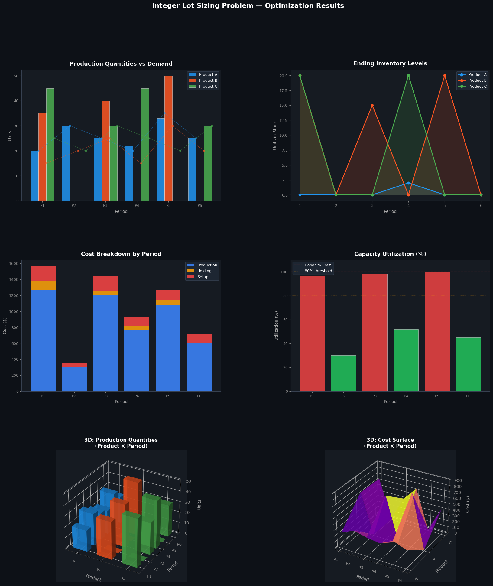

๐Ÿ“Š Graph Explanations

Plot 1 โ€” Production Quantities vs Demand

Grouped bars show how much is produced per product per period. Dashed marker lines overlay the actual demand. When a bar exceeds its demand marker, excess is being stored as inventory (intentional batching to amortize setup costs).

Plot 2 โ€” Ending Inventory Levels

Filled line charts reveal the inventory trajectory. A spike in period $t$ means the optimizer decided to batch-produce ahead of future demand, judging that the setup cost savings outweigh holding costs.

Plot 3 โ€” Cost Breakdown by Period (Stacked Bar)

Three cost components โ€” production (blue), holding (amber), setup (red) โ€” are stacked to show total period cost. Periods with no setup (no red) indicate the product was not produced that period.

Plot 4 โ€” Capacity Utilization

Bar height = percentage of capacity consumed. Green = comfortable headroom, red = near the limit. This validates that the capacity constraint $\sum_i a_i x_{it} \leq c_t$ is respected in every period.

Plot 5 โ€” 3D Bar: Production Quantities (Product ร— Period)

Each vertical bar represents $x_{it}$. The 3D view makes it immediately clear which product-period combinations receive production runs and how lot sizes vary across the planning horizon.

Plot 6 โ€” 3D Cost Surface (Product ร— Period)

A smooth plasma surface maps $p_i x_{it} + h_i s_{it} + f_i y_{it}$ for every $(i,t)$ cell. Peaks correspond to periods where a setup cost is incurred on top of large production runs. The surface geometry highlights the trade-off structure the solver is navigating.


๐Ÿ“‹ Execution Results

=======================================================
  Solver Status : Optimal
  Total Cost    : 6,274.00
=======================================================

โ”€โ”€ Production Plan (x_it) โ”€โ”€
Product        P1  P2  P3  P4  P5  P6
Product A       20   30   25   22   33   25
Product B       35    0   40    0   50    0
Product C       45    0   30   45    0   30

โ”€โ”€ Setup Decisions (y_it) โ”€โ”€
Product        P1  P2  P3  P4  P5  P6
Product A        1    1    1    1    1    1
Product B        1    0    1    0    1    0
Product C        1    0    1    1    0    1

โ”€โ”€ End Inventory (s_it) โ”€โ”€
Product        P1  P2  P3  P4  P5  P6
Product A        0    0    0    2    0    0
Product B       20    0   15    0   20    0
Product C       20    0    0   20    0    0

โ”€โ”€ Capacity Used / Available โ”€โ”€
  Period 1:    290 / 300  (96.7% utilization)
  Period 2:     90 / 300  (30.0% utilization)
  Period 3:    295 / 300  (98.3% utilization)
  Period 4:    156 / 300  (52.0% utilization)
  Period 5:    299 / 300  (99.7% utilization)
  Period 6:    135 / 300  (45.0% utilization)

[Figure saved as lot_sizing_results.png]

๐ŸŽฏ Key Takeaways

Why integer lots matter: Relaxing to continuous variables gives a lower-bound solution that may be infeasible in practice (e.g., 7.3 units of an indivisible component). The MIP guarantees all quantities are whole numbers.

Setup cost vs holding cost trade-off: The optimizer naturally consolidates production into fewer, larger runs when setup costs $f_i$ are high relative to holding costs $h_i$. You can experiment by increasing f and observe how the plan shifts toward longer batches.

Scalability: For this 3-product ร— 6-period instance, CBC solves in under a second. Real-world instances with hundreds of products and 52-week horizons may require commercial solvers (Gurobi, CPLEX) or heuristic methods (Lagrangian relaxation, column generation).