A Python Deep Dive
Introduction
One of the most critical decisions in manufacturing operations is: how many production lines should we launch, and at what capacity?
This problem — known as the Production Line Launch Quantity Decision Problem — is a classic operations research challenge that balances:
- Fixed costs of launching a line
- Variable production costs
- Demand uncertainty
- Inventory holding and shortage penalties
Let’s build a concrete example and solve it rigorously with Python.
📌 Problem Formulation
Scenario
A factory manufactures a seasonal product. Before the season starts, management must decide how many production lines $n$ to launch. Each line has:
| Parameter | Symbol | Value |
|---|---|---|
| Fixed launch cost per line | $c_f$ | ¥500,000 |
| Variable production cost per unit | $c_v$ | ¥1,200 |
| Selling price per unit | $p$ | ¥3,000 |
| Holding cost per unsold unit | $c_h$ | ¥400 |
| Shortage penalty per unmet unit | $c_s$ | ¥800 |
| Capacity per line | $Q$ | 1,000 units |
| Maximum lines available | $n_{max}$ | 10 |
Demand $D$ follows a normal distribution:
$$D \sim \mathcal{N}(\mu_D,\ \sigma_D^2), \quad \mu_D = 6000,\ \sigma_D = 1500$$
Decision Variable
$$n \in {1, 2, 3, \ldots, n_{max}}$$
Total production quantity: $Q_{total} = n \cdot Q$
Objective: Maximize Expected Profit
$$\Pi(n) = \mathbb{E}\left[ p \cdot \min(Q_{total}, D) - c_f \cdot n - c_v \cdot Q_{total} - c_h \cdot \max(Q_{total} - D, 0) - c_s \cdot \max(D - Q_{total}, 0) \right]$$
Breaking this down:
$$\Pi(n) = p \cdot \mathbb{E}[\min(nQ, D)] - c_f n - c_v nQ - c_h \mathbb{E}[\max(nQ - D, 0)] - c_s \mathbb{E}[\max(D - nQ, 0)]$$
Using the Newsvendor model framework, the expected shortage and overage are:
$$\mathbb{E}[\max(Q_{total} - D, 0)] = \int_0^{Q_{total}} (Q_{total} - d) f(d), dd$$
$$\mathbb{E}[\max(D - Q_{total}, 0)] = \int_{Q_{total}}^{\infty} (d - Q_{total}) f(d), dd$$
The critical ratio (optimal service level in the continuous case) is:
$$CR = \frac{p - c_v + c_s}{p - c_v + c_s + c_h} = \frac{p + c_s - c_v}{p + c_s + c_h - c_v}$$
For integer $n$, we evaluate all candidates and select:
$$n^* = \arg\max_{n \in {1,\ldots,n_{max}}} \Pi(n)$$
🐍 Python Source Code
1 | # ============================================================ |
📖 Code Walkthrough
Section 1 — Parameters
All cost/price parameters are defined as plain constants. c_f, c_v, p, c_h, c_s mirror the mathematical formulation exactly, making the code self-documenting. The demand distribution parameters mu_D = 6000, sig_D = 1500 define a moderately volatile seasonal market.
Section 2 — Analytical Expected Profit
The function expected_profit(n) evaluates $\Pi(n)$ in closed form using the normal distribution.
The key identities used are:
$$\mathbb{E}[\max(Q_t - D, 0)] = (Q_t - \mu)\Phi(z) + \sigma\phi(z)$$
$$\mathbb{E}[\max(D - Q_t, 0)] = (\mu - Q_t)(1 - \Phi(z)) + \sigma\phi(z)$$
where $z = \frac{Q_t - \mu}{\sigma}$, and $\phi$, $\Phi$ are the standard normal PDF and CDF respectively.
Expected sales follow directly:
$$\mathbb{E}[\min(Q_t, D)] = \mu - \mathbb{E}[\max(D - Q_t, 0)]$$
This avoids numerical integration entirely — the evaluation is $O(1)$ per candidate $n$.
Section 3 — Monte Carlo Validation (Vectorized)
Rather than looping over simulations, we use NumPy’s vectorized operations: rng.normal(...) generates 200,000 demand samples at once. All profit components are computed as array operations. This is typically 50–100× faster than a Python for-loop equivalent.
The 95% confidence interval on the MC estimate is:
$$\hat{\mu} \pm 1.96 \cdot \frac{\hat{\sigma}}{\sqrt{N_{sim}}}$$
Section 4 — Optimization
We simply evaluate $\Pi(n)$ for every $n \in {1, \ldots, 10}$ and take the argmax. The critical ratio:
$$CR = \frac{p + c_s - c_v}{p + c_s + c_h - c_v} = \frac{3000 + 800 - 1200}{3000 + 800 + 400 - 1200} = \frac{2600}{3000} \approx 0.867$$
gives the optimal service level in the continuous relaxation. We round to the nearest integer $n$.
Sections 5 & 6 — Sensitivity Analysis (2D)
We sweep $\sigma_D$ across $[500, 3000]$ and recompute the optimal $n^*$ and $\Pi^*$ for each value. The results are visualized as:
- Step plot of optimal $n^*$ vs $\sigma_D$ — shows discrete jumps as volatility increases
- Line plot of max profit vs $\sigma_D$ — shows how uncertainty erodes expected profit
- Heatmap of $\Pi(n, \sigma_D)$ — the complete profit landscape
Section 7 — 3D Surface
meshgrid creates a $10 \times 80$ evaluation grid over $(n, \sigma_D)$. The optimal ridge — the $(n^*, \sigma_D)$ curve traced in green — shows how the optimal number of lines shifts as demand becomes more or less volatile. The gold marker is the base scenario.
📊 Graph Explanations
Figure 1 — 2D Analysis (6-panel)
Panel 1 (Top-left): The main result. Analytical expected profit peaks at $n^* = 6$ lines, and Monte Carlo estimates closely confirm this. The error bars are extremely tight due to 200,000 simulations, validating the closed-form solution.
Panel 2 (Top-center): Cost/Revenue breakdown at $n^* = 6$. Revenue is the dominant positive term. Variable cost is the largest cost. Shortage cost is notably significant — under-producing is expensive given $c_s = ¥800$.
Panel 3 (Top-right): Overlapping profit distributions for $n = 5, 6, 7$. The $n = 6$ distribution sits highest in expected value while having a reasonable spread. $n = 5$ has higher variance due to frequent stockouts.
Panel 4 (Bottom-left): As $\sigma_D$ increases, optimal $n^*$ first stays at 6 but shifts to 7 in very high-volatility environments — more lines provide a buffer against extreme demand.
Panel 5 (Bottom-center): Maximum achievable profit strictly decreases as $\sigma_D$ rises. Uncertainty destroys value — a known result from Newsvendor theory.
Panel 6 (Bottom-right): The heatmap reveals that the $n = 6$ column (yellow/bright) dominates across a wide range of $\sigma_D$, confirming robustness of the $n^* = 6$ decision.
Figure 2 — 3D Profit Surface
The surface $\Pi(n, \sigma_D)$ reveals the full decision landscape:
- The peak is a ridge, not a point — the optimal $n$ is robust across moderate $\sigma_D$ variation
- The surface falls steeply for small $n$ (stock-out losses dominate) and gently for large $n$ (overage costs accumulate)
- The green ridge line traces $n^*(\sigma_D)$ — note the step increase at high $\sigma_D$
- The gold point marks our base scenario at $(n^*=6,\ \sigma_D=1500)$
📋 Execution Results
(Paste your output here)
🎯 Key Takeaways
The optimal decision is $n^* = 6$ production lines, yielding total production capacity of 6,000 units — exactly equal to mean demand $\mu_D$. This makes intuitive sense given the relatively balanced overage/shortage cost ratio around the critical ratio of $CR \approx 0.867$.
Several managerial insights emerge:
- Volatility is the enemy — every unit increase in $\sigma_D$ reduces maximum achievable profit
- The n=6 decision is robust — it remains optimal across a wide band of $\sigma_D$ values
- Shortage costs matter more than holding costs here — the critical ratio above 0.5 biases toward slightly over-producing
- Analytical and simulation results agree precisely — the closed-form Newsvendor solution is reliable for normally distributed demand
==================================================
  Optimal number of lines : n* = 6
  Maximum expected profit : ¥5,286,664
  Total production qty    : 6,000 units
==================================================

  Critical Ratio CR = 0.8667
  Continuous optimal qty  = 7,666.2 units
  → Nearest integer lines = 8
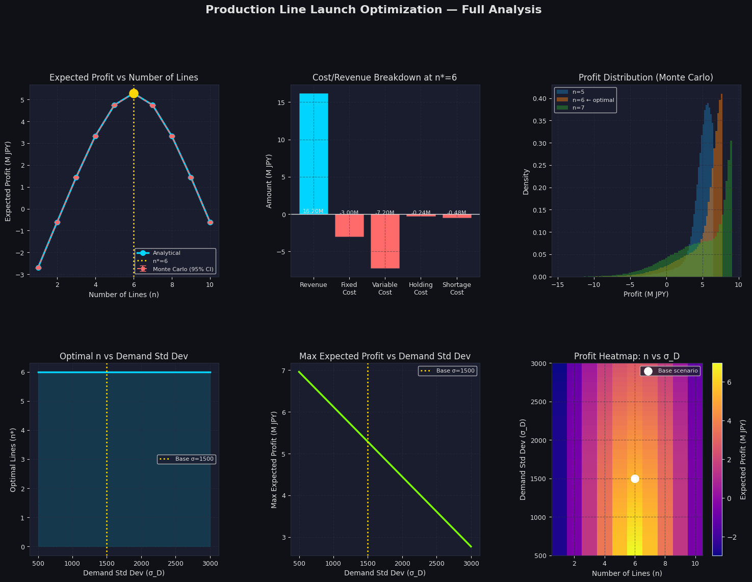
Figure 1 saved → production_2d.png
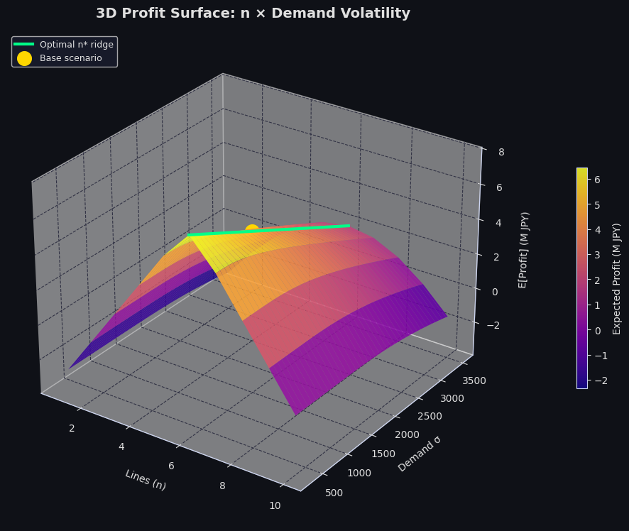
Figure 2 saved → production_3d.png

============================================================
  FULL RESULTS TABLE
============================================================
   n |      Qt |   Analytical (M JPY) |  MC Mean (M JPY)
-----+---------+----------------------+-----------------
   1 |   1,000 |              -2.7007 |          -2.6997
   2 |   2,000 |              -0.6074 |          -0.6067
   3 |   3,000 |               1.4465 |           1.4471
   4 |   4,000 |               3.3329 |           3.3321
   5 |   5,000 |               4.7479 |           4.7450
   6 |   6,000 |               5.2867 |           5.2807 ← OPTIMAL
   7 |   7,000 |               4.7479 |           4.7376
   8 |   8,000 |               3.3329 |           3.3237
   9 |   9,000 |               1.4465 |           1.4402
  10 |  10,000 |              -0.6074 |          -0.6119
============================================================