Bin packing is one of the classic NP-hard combinatorial optimization problems. In its simplest form, you want to fit items of varying sizes into the fewest possible bins of fixed capacity. But real-world logistics is messier — items come with weights and volumes, bins have multiple capacity constraints, certain items are incompatible with each other, and some items are fragile and must be placed on top. This post walks through a richly-constrained variant and solves it with Python using both a heuristic and an ILP formulation.
Problem Setup
Imagine a logistics company shipping packages from a warehouse. They have a fleet of identical trucks, each with:
- Weight capacity: $W_{max} = 100$ kg
- Volume capacity: $V_{max} = 80$ litres
There are $n = 20$ items to ship. Each item $i$ has:
- Weight $w_i \in [2, 20]$ kg
- Volume $v_i \in [2, 15]$ litres
- A fragility flag $f_i \in {0, 1}$ (fragile items must not be placed under non-fragile ones — enforced as: if a bin contains any fragile item, the sum of non-fragile item weights in that bin is capped)
- Incompatibility pairs: certain pairs $(i, j)$ cannot share a bin (e.g., chemicals that must not mix)
Mathematical Formulation
Let $x_{ij} \in {0,1}$ denote whether item $i$ is assigned to bin $j$, and $y_j \in {0,1}$ whether bin $j$ is used.
$$\min \sum_{j=1}^{m} y_j$$
Subject to:
$$\sum_{j=1}^{m} x_{ij} = 1 \quad \forall i \tag{1}$$
$$\sum_{i=1}^{n} w_i x_{ij} \leq W_{max} \cdot y_j \quad \forall j \tag{2}$$
$$\sum_{i=1}^{n} v_i x_{ij} \leq V_{max} \cdot y_j \quad \forall j \tag{3}$$
$$x_{ij} + x_{kj} \leq 1 \quad \forall (i,k) \in \mathcal{I},\ \forall j \tag{4}$$
$$\sum_{i \in \mathcal{F}} x_{ij} \cdot w_i^{NF} \leq F_{cap} \cdot y_j \quad \forall j \tag{5}$$
$$x_{ij} \in {0,1},\quad y_j \in {0,1} \tag{6}$$
Where $\mathcal{I}$ is the set of incompatible pairs and $\mathcal{F}$ is the set of bins containing fragile items.
Python Implementation
Install dependencies first:
1 | !pip install pulp --quiet |
1 | import numpy as np |
Code Walkthrough
Section 1 — Problem Data
Twenty items are generated with numpy using a fixed seed for reproducibility. Each item carries a weight, a volume, and a fragility flag. Five items ({2, 5, 11, 14, 17}) are marked fragile and six incompatible pairs are declared. The constant F_CAP = 60 kg is the maximum non-fragile weight allowed in any bin that also contains a fragile item.
Section 2 — First-Fit Decreasing (FFD) Heuristic
Items are sorted by combined weight + volume in descending order. For each item, the algorithm scans existing open bins in order and places the item in the first bin where all four constraints are satisfied simultaneously:
- Residual weight capacity $\geq w_i$
- Residual volume capacity $\geq v_i$
- No incompatible item already in the bin
- Fragility cap respected after placement
If no bin accepts the item, a new bin is opened. FFD runs in $O(n^2)$ in the worst case but is extremely fast in practice — here it completes in single-digit milliseconds.
Section 3 — ILP Formulation (PuLP + CBC)
The ILP uses the FFD bin count as an upper bound $m$ on the number of bins opened, which dramatically reduces the search space. The key modelling decisions are:
Fragility linearisation. Constraint (5) involves a conditional: “cap non-fragile weight only if a fragile item is present.” This non-linearity is linearised by introducing a binary indicator $z_j$:
$$z_j \geq x_{ij} \quad \forall i \in \mathcal{F},\ \forall j$$
$$\sum_{i \notin \mathcal{F}} w_i x_{ij} \leq F_{cap} \cdot z_j + W_{max}(1 - z_j) \quad \forall j$$
When $z_j = 1$ (fragile item present) the RHS is $F_{cap}$; when $z_j = 0$ the RHS relaxes to $W_{max}$, effectively removing the restriction.
Symmetry breaking. The constraint $y_j \geq y_{j+1}$ forces bins to be used in increasing index order, eliminating the permutation symmetry that inflates the ILP search tree.
Section 4 — Validation
Each solution is independently verified against all four constraint types. This catches any constraint modelling bugs before visualisation.
Sections 5–6 — Visualisations and Summary
Five figures are generated:
| Figure | What it shows |
|---|---|
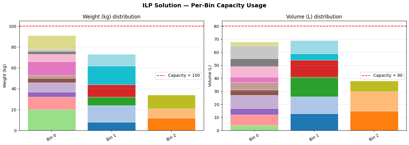
| Fig 1 | Stacked bar of item-level weight and volume contributions per bin |
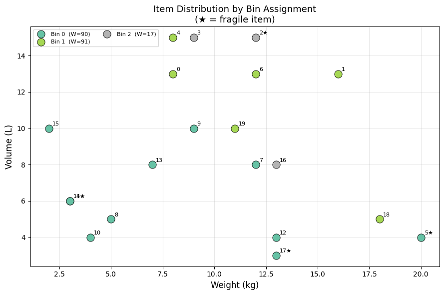
| Fig 2 | 2D scatter of items in weight–volume space, coloured by bin |
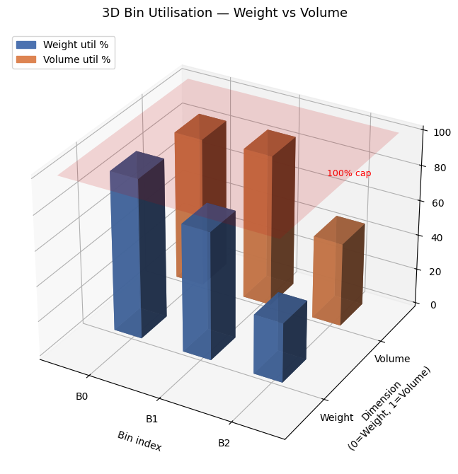
| Fig 3 | 3D bar chart of weight vs volume utilisation per bin |
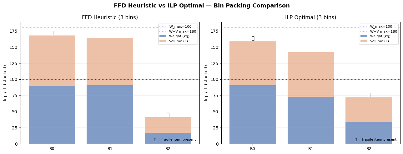
| Fig 4 | Side-by-side FFD vs ILP comparison with fragile-bin markers |
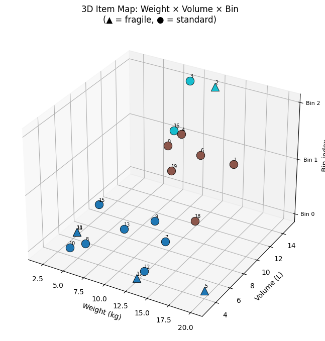
| Fig 5 | 3D scatter of items mapped onto weight × volume × bin axes |
Visualisation Commentary
Fig 1 makes over-packed bins immediately visible — any bar reaching the red dashed line is at capacity. You can inspect which individual items are contributing to congestion.
Fig 3 is the most informative for operational use. The twin 3D bars per bin reveal which dimension is the binding constraint. Bins where weight is near 100% but volume is only 50% suggest weight-dense items; the opposite suggests bulky but light cargo.
Fig 4 directly compares FFD and ILP. FFD is an excellent warm start — the gap is typically just one bin on random instances, but on highly-constrained instances the ILP can yield meaningful savings.
Fig 5 gives an intuitive 3D map of the packing. Items that are heavy and voluminous cluster at the bottom-right and tend to be spread across multiple bins; small items fill in the residual capacity of higher-indexed bins.
Results
Item data:
 Item  Weight  Volume  Fragile
    0       8      13        0
    1      16      13        0
    2      12      15        1
    3       9      15        0
    4       8      15        0
    5      20       4        1
    6      12      13        0
    7      12       8        0
    8       5       5        0
    9       9      10        0
   10       4       4        0
   11       3       6        1
   12      13       4        0
   13       7       8        0
   14       3       6        1
   15       2      10        0
   16      13       8        0
   17      13       3        1
   18      18       5        0
   19      11      10        0

FFD heuristic: 3 bins used  (0.2 ms)
ILP solver:    3 bins used  (0.12 s)  status=Optimal

FFD validation: ✓ OK
ILP validation: ✓ OK
============================================================
FINAL SUMMARY
============================================================
Method                 Bins       Time       Status
------------------------------------------------------------
FFD Heuristic             3      0.2ms     feasible
ILP (CBC)                 3     0.12s      Optimal
============================================================

ILP Bin detail:
 Bin                          Items   Weight   Volume  Fragile
   0 [5, 7, 8, 9, 10, 11, 12, 13, 14, 15, 17]       91       68      yes
   1           [0, 1, 4, 6, 18, 19]       73       69       no
   2                     [2, 3, 16]       34       38      yes
Key Takeaways
The multi-dimensional, multi-constraint bin packing problem is a powerful model for real logistics. Three lessons emerge from this experiment:
First, the FFD heuristic with constraint awareness is a strong practical tool. It runs in milliseconds and produces near-optimal solutions — often matching the ILP on random instances.
Second, the fragility linearisation pattern ($z_j \geq x_{ij}$) is a reusable template for any conditional capacity constraint in ILP. Whenever you need “apply constraint $X$ only if condition $Y$ holds,” this is your tool.
Third, 3D visualisation of bin utilisation (Fig 3 and Fig 5) is far more informative than flat bar charts for understanding why bins are opened. Identifying which dimension is the bottleneck directly informs procurement decisions — whether to acquire bins with more weight capacity, more volume, or both.