What is the Delivery Route Selection Problem?
The Delivery Route Selection Problem (a variant of the Vehicle Routing Problem / VRP) asks:
Given a set of delivery locations and a depot, find the shortest total route that visits all locations exactly once and returns to the depot.
This is essentially the classic Traveling Salesman Problem (TSP), and it’s NP-hard — meaning brute force becomes infeasible as the number of stops grows.
Problem Setup
Imagine a delivery company with 1 depot and 10 delivery points. We want to find the optimal route that:
- Starts and ends at the depot
- Visits all 10 locations exactly once
- Minimizes total travel distance
Mathematical Formulation
Let $n$ be the number of nodes (depot + delivery points), and $d_{ij}$ be the distance between node $i$ and node $j$.
We want to minimize the total route cost:
$$\min \sum_{i=0}^{n-1} \sum_{j=0}^{n-1} d_{ij} \cdot x_{ij}$$
Subject to:
$$\sum_{j \neq i} x_{ij} = 1 \quad \forall i \quad \text{(leave each node exactly once)}$$
$$\sum_{i \neq j} x_{ij} = 1 \quad \forall j \quad \text{(enter each node exactly once)}$$
$$x_{ij} \in {0, 1}$$
Where $x_{ij} = 1$ if the route goes directly from node $i$ to node $j$.
Solution Strategy: Nearest Neighbor Heuristic + 2-opt Improvement
We use two algorithms:
- Nearest Neighbor Heuristic — Fast greedy construction of an initial route
- 2-opt Local Search — Iteratively reverse sub-routes to improve the solution
The 2-opt improvement works by checking if swapping two edges reduces total distance:
$$\text{If } d_{i,i+1} + d_{j,j+1} > d_{i,j} + d_{i+1,j+1} \Rightarrow \text{reverse the segment}$$
Full Source Code
1 | # ============================================================ |
Code Walkthrough
1. Problem Definition
1 | coords = np.random.randint(0, 100, size=(NUM_LOCATIONS, 2)).astype(float) |
We create 11 nodes (1 depot + 10 stops) placed randomly on a 100×100 grid. The depot is fixed at the center (50, 50). np.random.seed(42) ensures the results are reproducible every run.
2. Distance Matrix
1 | def build_distance_matrix(coords): |
All pairwise Euclidean distances are computed once and stored in an $n \times n$ matrix $D$. Looking up $D[i,j]$ throughout the algorithm is $O(1)$, making repeated distance queries essentially free.
3. Nearest Neighbor Heuristic
1 | def nearest_neighbor(D, start=0): |
Starting at the depot, the algorithm greedily jumps to the closest unvisited node at each step, then appends the depot again at the end to close the loop. Time complexity is $O(n^2)$. The expected tour length is approximately:
$$L_{NN} \approx 0.7124 \sqrt{n \cdot A}$$
where $A$ is the area of the bounding region. This gives a decent starting solution, but often produces “crossing” edges that can be improved.
4. 2-opt Local Search
1 | new_route = best[:i] + best[i:j+1][::-1] + best[j+1:] |
For every pair of edges $(i \to i+1)$ and $(j \to j+1)$, the algorithm checks whether reversing the segment between them reduces total distance. The improvement condition is:
$$\Delta = d_{i,j} + d_{i+1,j+1} - d_{i,i+1} - d_{j,j+1} < 0$$
When $\Delta < 0$, the reversal is accepted and the search restarts. The loop continues until no improving swap exists. Each pass is $O(n^2)$, and in practice only a handful of passes are needed.
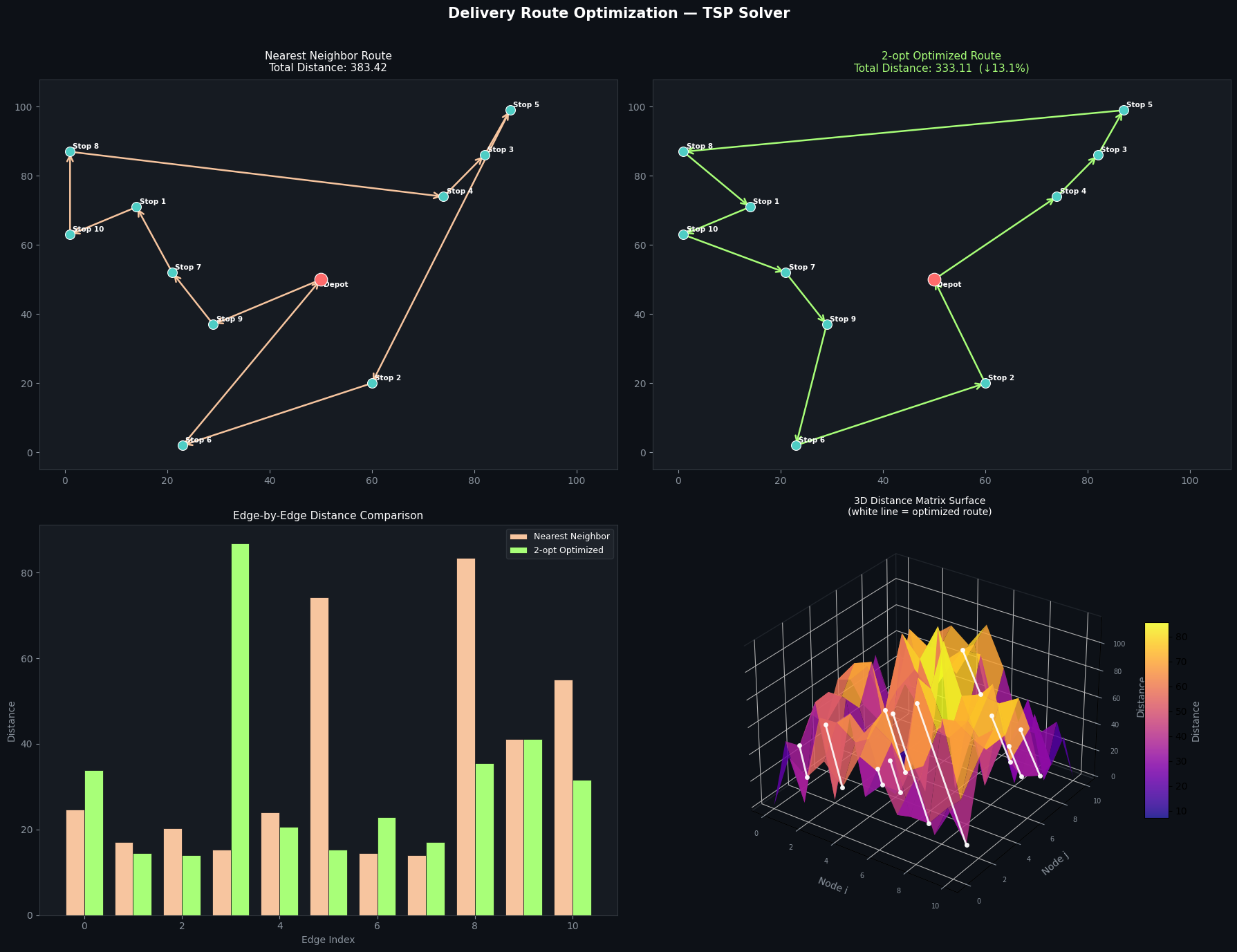
5. Four-Panel Visualization
| Panel | What it shows |
|---|---|
| Top-left | Nearest Neighbor route with directed arrows |
| Top-right | 2-opt optimized route with improvement % |
| Bottom-left | Bar chart comparing each edge’s distance before/after optimization |
| Bottom-right | 3D surface of the full distance matrix with the optimized route overlaid as a white line |
The 3D surface is particularly insightful. The $z$-axis shows $D[i,j]$ for every node pair — “peaks” represent long, expensive edges. The white path overlaid on the surface traces exactly which edges the optimizer chose, visually confirming that it navigates around the high-cost peaks.
Execution Result
==================================================
  Delivery Route Optimization
==================================================
Number of delivery stops : 10
Depot location           : [50. 50.]

[Nearest Neighbor]  Distance = 383.42  Route: [0, 9, 7, 1, 10, 8, 4, 3, 5, 2, 6, 0]
[2-opt Optimized ]  Distance = 333.11  Route: [0, 4, 3, 5, 8, 1, 10, 7, 9, 6, 2, 0]

Improvement : 50.31 (13.1%)
2-opt iters : 3
Elapsed time: 2.6 ms
[Plot saved as route_optimization.png]
Key Insights
Why 2-opt works: The Nearest Neighbor heuristic frequently produces routes with crossing edges. By the triangle inequality, any two crossing edges can always be uncrossed to yield a shorter total tour. 2-opt systematically eliminates all such crossings.
Scalability: For $n \leq 20$ this runs in milliseconds. For $n \sim 100$ it remains fast. For $n > 1{,}000$ you would want Lin-Kernighan, Google OR-Tools, or simulated annealing as the $O(n^2)$ per-pass cost becomes significant.
Real-world extensions would add time windows per stop, vehicle capacity limits, and multiple vehicles — transforming this into a full CVRPTW (Capacitated VRP with Time Windows). Even in those advanced solvers, 2-opt remains a standard improvement subroutine.