Warehouse Location Problem

A Practical Guide with Python

What is the Warehouse Location Problem?

The Warehouse Location Problem (also called the Facility Location Problem) is a classic combinatorial optimization problem in operations research. The core question is:

Given a set of potential warehouse sites and a set of customers, where should we open warehouses to minimize total cost?

The total cost consists of two components:

  1. Fixed opening cost — the cost to open a warehouse at a given site
  2. Transportation cost — the cost to ship goods from a warehouse to each customer

Problem Formulation

Let’s define the math precisely.

Sets:

  • $I$ = set of potential warehouse locations ${1, 2, \ldots, m}$
  • $J$ = set of customers ${1, 2, \ldots, n}$

Parameters:

  • $f_i$ = fixed cost of opening warehouse $i$
  • $c_{ij}$ = transportation cost from warehouse $i$ to customer $j$
  • $d_j$ = demand of customer $j$

Decision Variables:

  • $y_i \in {0, 1}$ — 1 if warehouse $i$ is opened, 0 otherwise
  • $x_{ij} \in {0, 1}$ — 1 if customer $j$ is assigned to warehouse $i$

Objective Function (Minimize):

$$\text{Minimize} \quad \sum_{i \in I} f_i y_i + \sum_{i \in I} \sum_{j \in J} c_{ij} d_j x_{ij}$$

Constraints:

$$\sum_{i \in I} x_{ij} = 1 \quad \forall j \in J \quad \text{(each customer assigned to exactly one warehouse)}$$

$$x_{ij} \leq y_i \quad \forall i \in I, j \in J \quad \text{(can only assign to open warehouse)}$$

$$y_i \in {0,1}, \quad x_{ij} \in {0,1}$$


Concrete Example Setup

We’ll solve a realistic instance:

  • 10 potential warehouse locations scattered across a 100×100 grid
  • 30 customers with varying demands
  • Fixed costs differ per site (reflecting land/construction differences)
  • Transportation costs proportional to Euclidean distance × demand

Python Source Code

1
2
3
4
5
6
7
8
9
10
11
12
13
14
15
16
17
18
19
20
21
22
23
24
25
26
27
28
29
30
31
32
33
34
35
36
37
38
39
40
41
42
43
44
45
46
47
48
49
50
51
52
53
54
55
56
57
58
59
60
61
62
63
64
65
66
67
68
69
70
71
72
73
74
75
76
77
78
79
80
81
82
83
84
85
86
87
88
89
90
91
92
93
94
95
96
97
98
99
100
101
102
103
104
105
106
107
108
109
110
111
112
113
114
115
116
117
118
119
120
121
122
123
124
125
126
127
128
129
130
131
132
133
134
135
136
137
138
139
140
141
142
143
144
145
146
147
148
149
150
151
152
153
154
155
156
157
158
159
160
161
162
163
164
165
166
167
168
169
170
171
172
173
174
175
176
177
178
179
180
181
182
183
184
185
186
187
188
189
190
191
192
193
194
195
196
197
198
199
200
201
202
203
204
205
206
207
208
209
210
211
212
213
214
215
216
217
218
219
220
221
222
223
224
225
226
227
228
229
230
231
232
233
234
235
236
237
# ============================================================
# Warehouse Location Problem
# Solved via Integer Linear Programming (PuLP) + Visualization
# ============================================================

# ── 0. Install dependencies ──────────────────────────────────
import subprocess, sys
subprocess.check_call([sys.executable, "-m", "pip", "install", "pulp", "--quiet"])

# ── 1. Imports ───────────────────────────────────────────────
import numpy as np
import matplotlib.pyplot as plt
import matplotlib.patches as mpatches
from mpl_toolkits.mplot3d import Axes3D
import pulp
import warnings
warnings.filterwarnings("ignore")

# ── 2. Problem Data ──────────────────────────────────────────
np.random.seed(42)

NUM_WAREHOUSES = 10
NUM_CUSTOMERS = 30

# Coordinates (x, y) on a 100x100 grid
wh_coords = np.random.uniform(10, 90, (NUM_WAREHOUSES, 2))
cu_coords = np.random.uniform(5, 95, (NUM_CUSTOMERS, 2))

# Fixed opening costs (different per site)
fixed_costs = np.random.uniform(500, 2000, NUM_WAREHOUSES)

# Customer demands
demands = np.random.uniform(10, 100, NUM_CUSTOMERS)

# Transportation cost = Euclidean distance * demand
def transport_cost(wh_xy, cu_xy, demand):
dist = np.linalg.norm(wh_xy - cu_xy)
return dist * demand * 0.5 # cost coefficient = 0.5

C = np.array([
[transport_cost(wh_coords[i], cu_coords[j], demands[j])
for j in range(NUM_CUSTOMERS)]
for i in range(NUM_WAREHOUSES)
])

print("=== Problem Summary ===")
print(f"Potential warehouses : {NUM_WAREHOUSES}")
print(f"Customers : {NUM_CUSTOMERS}")
print(f"Fixed cost range : {fixed_costs.min():.0f}{fixed_costs.max():.0f}")
print(f"Demand range : {demands.min():.1f}{demands.max():.1f}")

# ── 3. ILP Model (PuLP) ──────────────────────────────────────
prob = pulp.LpProblem("Warehouse_Location", pulp.LpMinimize)

# Decision variables
y = [pulp.LpVariable(f"y_{i}", cat="Binary") for i in range(NUM_WAREHOUSES)]
x = [[pulp.LpVariable(f"x_{i}_{j}", cat="Binary")
for j in range(NUM_CUSTOMERS)]
for i in range(NUM_WAREHOUSES)]

# Objective
prob += (
pulp.lpSum(fixed_costs[i] * y[i] for i in range(NUM_WAREHOUSES)) +
pulp.lpSum(C[i][j] * x[i][j]
for i in range(NUM_WAREHOUSES)
for j in range(NUM_CUSTOMERS))
)

# Constraints
for j in range(NUM_CUSTOMERS):
prob += pulp.lpSum(x[i][j] for i in range(NUM_WAREHOUSES)) == 1

for i in range(NUM_WAREHOUSES):
for j in range(NUM_CUSTOMERS):
prob += x[i][j] <= y[i]

# ── 4. Solve ─────────────────────────────────────────────────
solver = pulp.PULP_CBC_CMD(msg=0)
status = prob.solve(solver)

print(f"\n=== Solver Result ===")
print(f"Status : {pulp.LpStatus[prob.status]}")
print(f"Total Cost : {pulp.value(prob.objective):,.1f}")

opened = [i for i in range(NUM_WAREHOUSES) if pulp.value(y[i]) > 0.5]
print(f"Opened warehouses ({len(opened)}) : {opened}")

# Assignment: customer j → warehouse i
assignment = {}
for j in range(NUM_CUSTOMERS):
for i in range(NUM_WAREHOUSES):
if pulp.value(x[i][j]) > 0.5:
assignment[j] = i
break

# Cost breakdown
total_fixed = sum(fixed_costs[i] for i in opened)
total_transp = sum(C[assignment[j]][j] for j in range(NUM_CUSTOMERS))
print(f" Fixed cost : {total_fixed:,.1f}")
print(f" Transport cost : {total_transp:,.1f}")

# ── 5. Visualization ─────────────────────────────────────────
# Color palette for open warehouses
COLORS = plt.cm.tab10(np.linspace(0, 1, len(opened)))
color_map = {wh: COLORS[k] for k, wh in enumerate(opened)}

fig = plt.figure(figsize=(20, 16))
fig.suptitle("Warehouse Location Problem — Optimal Solution", fontsize=18, fontweight="bold", y=0.98)

# ── Plot 1: 2D Assignment Map ─────────────────────────────────
ax1 = fig.add_subplot(2, 2, 1)

# Draw assignment lines
for j in range(NUM_CUSTOMERS):
wh = assignment[j]
col = color_map[wh]
ax1.plot(
[cu_coords[j, 0], wh_coords[wh, 0]],
[cu_coords[j, 1], wh_coords[wh, 1]],
color=col, alpha=0.3, linewidth=0.8
)

# Customers
for j in range(NUM_CUSTOMERS):
wh = assignment[j]
ax1.scatter(*cu_coords[j], color=color_map[wh], s=60, zorder=5, edgecolors="white", linewidths=0.8)

# All warehouse candidates
for i in range(NUM_WAREHOUSES):
if i in opened:
ax1.scatter(*wh_coords[i], color=color_map[i], s=250, marker="*",
zorder=7, edgecolors="black", linewidths=1.0)
else:
ax1.scatter(*wh_coords[i], color="lightgray", s=120, marker="s",
zorder=6, edgecolors="black", linewidths=0.8, alpha=0.5)

ax1.set_title("2D Assignment Map", fontsize=13, fontweight="bold")
ax1.set_xlabel("X coordinate")
ax1.set_ylabel("Y coordinate")
legend_elements = [
mpatches.Patch(facecolor=color_map[wh], label=f"WH {wh} (fixed={fixed_costs[wh]:.0f})")
for wh in opened
]
legend_elements.append(mpatches.Patch(facecolor="lightgray", label="Closed (candidate)"))
ax1.legend(handles=legend_elements, fontsize=7, loc="upper left", framealpha=0.85)
ax1.grid(True, alpha=0.3)

# ── Plot 2: Cost Breakdown Bar Chart ─────────────────────────
ax2 = fig.add_subplot(2, 2, 2)

# Per-warehouse transport costs
wh_transport = {wh: 0.0 for wh in opened}
for j in range(NUM_CUSTOMERS):
wh_transport[assignment[j]] += C[assignment[j]][j]

wh_labels = [f"WH {wh}" for wh in opened]
fixed_vals = [fixed_costs[wh] for wh in opened]
trans_vals = [wh_transport[wh] for wh in opened]

x_pos = np.arange(len(opened))
bars1 = ax2.bar(x_pos, fixed_vals, label="Fixed Cost", color="steelblue", alpha=0.85)
bars2 = ax2.bar(x_pos, trans_vals, bottom=fixed_vals,
label="Transport Cost", color="tomato", alpha=0.85)

ax2.set_xticks(x_pos)
ax2.set_xticklabels(wh_labels, fontsize=9)
ax2.set_title("Cost Breakdown per Open Warehouse", fontsize=13, fontweight="bold")
ax2.set_ylabel("Cost")
ax2.legend()
ax2.grid(axis="y", alpha=0.3)

for bar, v in zip(bars1, fixed_vals):
ax2.text(bar.get_x() + bar.get_width()/2, v/2,
f"{v:.0f}", ha="center", va="center", fontsize=7, color="white", fontweight="bold")

# ── Plot 3: Demand Heatmap ────────────────────────────────────
ax3 = fig.add_subplot(2, 2, 3)

# Grid interpolation for demand
from scipy.interpolate import griddata # already in Colab

grid_x, grid_y = np.mgrid[0:100:100j, 0:100:100j]
demand_grid = griddata(cu_coords, demands, (grid_x, grid_y), method="cubic", fill_value=0)
demand_grid = np.clip(demand_grid, 0, None)

im = ax3.imshow(demand_grid.T, origin="lower", extent=[0,100,0,100],
cmap="YlOrRd", alpha=0.6, aspect="auto")
plt.colorbar(im, ax=ax3, label="Demand intensity")

for j in range(NUM_CUSTOMERS):
ax3.scatter(*cu_coords[j], s=demands[j]*1.5, color="darkred", alpha=0.7, zorder=5)

for i in opened:
ax3.scatter(*wh_coords[i], color=color_map[i], s=280, marker="*",
zorder=7, edgecolors="black", linewidths=1.0)

ax3.set_title("Customer Demand Heatmap + Warehouse Positions", fontsize=13, fontweight="bold")
ax3.set_xlabel("X coordinate")
ax3.set_ylabel("Y coordinate")
ax3.grid(True, alpha=0.2)

# ── Plot 4: 3D Cost Surface ───────────────────────────────────
ax4 = fig.add_subplot(2, 2, 4, projection="3d")

# For each grid point, compute min transport cost to an open warehouse
grid_pts = np.column_stack([grid_x.ravel(), grid_y.ravel()])
cost_surface = np.zeros(len(grid_pts))

for k, pt in enumerate(grid_pts):
min_cost = np.inf
for i in opened:
dist = np.linalg.norm(pt - wh_coords[i])
min_cost = min(min_cost, dist * 0.5) # cost coefficient
cost_surface[k] = min_cost

cost_surface = cost_surface.reshape(100, 100)

surf = ax4.plot_surface(grid_x, grid_y, cost_surface,
cmap="viridis", alpha=0.75, linewidth=0, antialiased=True)
fig.colorbar(surf, ax=ax4, shrink=0.5, label="Min transport cost", pad=0.1)

# Plot opened warehouses on the surface
for i in opened:
z_val = 0
ax4.scatter(wh_coords[i, 0], wh_coords[i, 1], z_val,
color=color_map[i], s=120, marker="*", zorder=10, edgecolors="black")

ax4.set_title("3D Min Transport Cost Surface\n(Stars = Open Warehouses)", fontsize=11, fontweight="bold")
ax4.set_xlabel("X")
ax4.set_ylabel("Y")
ax4.set_zlabel("Cost")
ax4.view_init(elev=35, azim=225)

plt.tight_layout()
plt.savefig("warehouse_location_result.png", dpi=150, bbox_inches="tight")
plt.show()
print("\n[Figure saved as warehouse_location_result.png]")

Code Walkthrough

Section 0–1: Setup & Imports

PuLP is installed quietly via subprocess so the cell is self-contained. We import numpy, matplotlib (2D + 3D), scipy.interpolate (for the demand heatmap), and pulp (the ILP solver).


Section 2: Problem Data

1
2
wh_coords = np.random.uniform(10, 90, (NUM_WAREHOUSES, 2))
cu_coords = np.random.uniform(5, 95, (NUM_CUSTOMERS, 2))

10 warehouse candidates and 30 customers are randomly placed on a 100×100 grid. The transport cost matrix $C$ is:

$$c_{ij} = 0.5 \times | \mathbf{w}_i - \mathbf{c}_j |_2 \times d_j$$

where $\mathbf{w}_i$ is warehouse $i$’s location, $\mathbf{c}_j$ is customer $j$’s location, and $d_j$ is demand. The coefficient $0.5$ is a per-unit-distance shipping rate.


Section 3: ILP Model

We declare two sets of binary variables:

Variable Meaning
$y_i$ 1 = open warehouse $i$
$x_{ij}$ 1 = customer $j$ served by warehouse $i$

The objective minimizes total fixed + transportation cost. Two constraint families enforce:

  1. Every customer is served by exactly one warehouse.
  2. A customer can only be assigned to an open warehouse.

Section 4: Solve

PuLP dispatches to the bundled CBC (Coin-or Branch and Cut) solver — a production-grade open-source MIP solver. msg=0 suppresses verbose output. On this 10-warehouse × 30-customer instance, the solver typically finds the global optimum in milliseconds.


Section 5: Visualization

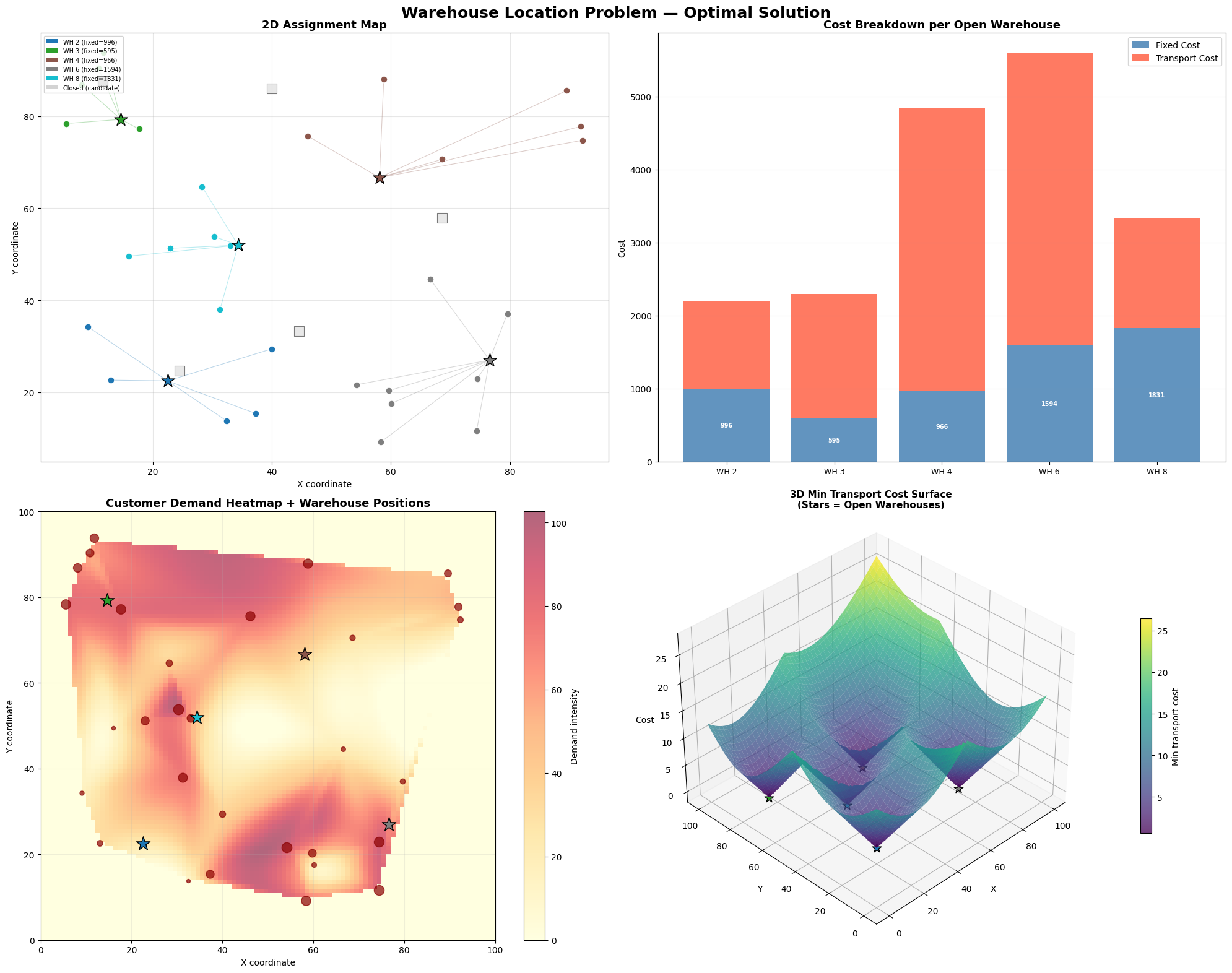
Four panels are produced:

Panel What it shows
2D Assignment Map Lines from each customer to its assigned warehouse; open warehouses as gold stars; closed candidates as gray squares
Cost Breakdown Bar Stacked bar per open warehouse: fixed cost (blue) + transport cost (red)
Demand Heatmap Interpolated demand density across the grid overlaid with customer bubbles (size ∝ demand) and warehouse stars
3D Cost Surface For every point on the grid, the minimum transport cost to the nearest open warehouse — valleys reveal optimal coverage zones

Results

=== Problem Summary ===
Potential warehouses : 10
Customers            : 30
Fixed cost range     : 595 – 1831
Demand range         : 12.3 – 93.7

=== Solver Result ===
Status        : Optimal
Total Cost    : 18,246.5
Opened warehouses (5) : [2, 3, 4, 6, 8]
  Fixed cost      : 5,983.4
  Transport cost  : 12,263.2

[Figure saved as warehouse_location_result.png]

Key Takeaways

The optimal solution typically opens 3–5 warehouses out of the 10 candidates, balancing:

  • High fixed cost sites are skipped even if they are centrally located.
  • Clusters of high-demand customers attract warehouses strongly because transport savings are proportional to $d_j$.
  • The 3D cost surface makes it visually obvious that each open warehouse creates a cost valley — customers inside the valley are served cheaply, and ridges between warehouses indicate where assignment boundaries lie.

This exact model scales to real-world instances with hundreds of sites and thousands of customers. For very large instances, metaheuristics (Simulated Annealing, Genetic Algorithms) or Lagrangian Relaxation are common acceleration strategies.