🧮 Solved with Python (Integer Programming)
What Is the Project Selection Problem?
The Project Selection Problem is a classic combinatorial optimization problem. You have a set of candidate projects, each with a profit and a cost, and some projects have dependencies (you can’t do Project B unless you first do Project A). Given a fixed budget, the goal is to select a subset of projects that maximizes total profit while satisfying all dependency constraints and the budget constraint.
Concrete Example
Suppose a company has 6 candidate projects:
| Project | Profit | Cost | Prerequisite |
|---|---|---|---|
| P1 | 10 | 3 | — |
| P2 | 20 | 5 | P1 |
| P3 | 15 | 4 | P1 |
| P4 | 25 | 7 | P2 |
| P5 | 18 | 6 | P3 |
| P6 | 30 | 8 | P2, P3 |
Budget: 20 units
Mathematical Formulation
Let $x_i \in {0, 1}$ be a binary decision variable: $x_i = 1$ if project $i$ is selected.
Objective (Maximize total profit):
$$\max \sum_{i=1}^{n} p_i x_i$$
Budget constraint:
$$\sum_{i=1}^{n} c_i x_i \leq B$$
Dependency constraints (if project $j$ requires project $i$):
$$x_j \leq x_i \quad \forall (i, j) \in E$$
where $E$ is the set of prerequisite edges.
Python Source Code
1 | # ============================================================ |
Code Walkthrough
Section 1 — Problem Definition
All six projects are stored in a Python dictionary. Each entry holds three keys: profit, cost, and prereqs (a list of prerequisite project names). The budget is set as the constant BUDGET = 20.
Section 2 — ILP Model with PuLP
PuLP is Python’s standard library for Linear / Integer Programming.
- A binary variable $x_i$ is created for every project via
pulp.LpVariable(..., cat='Binary'). - The objective is declared with
pulp.lpSum(...), which maps directly to $\max \sum p_i x_i$. - The budget constraint sums all selected project costs and requires the total $\leq 20$.
- Dependency constraints enforce $x_j \leq x_i$: selecting a child project forces its prerequisite to be selected as well.
PULP_CBC_CMD(msg=0)invokes the open-source CBC solver silently.
Section 3 — Print Results
Selected projects, total profit, total cost, remaining budget, and solver status are printed to the console in a formatted block.
Section 4 — Brute-Force Enumeration
With only $n = 6$ projects there are $2^6 = 64$ subsets — small enough for exhaustive search. Every combination is checked for budget feasibility and dependency validity. This produces the complete list of feasible portfolios used in the charts.
Section 5 — Four Visualizations
Plot 1 — Dependency Graph renders the prerequisite DAG using networkx. Cyan nodes are selected; pink nodes are rejected. Each node shows profit and cost inline.
Plot 2 — Profit vs Cost Scatter plots every feasible combination as a bubble. Bubble size encodes the number of projects in that portfolio. The gold star marks the optimal solution; the red dashed line marks the budget ceiling.
Plot 3 — 3D Scatter adds a third axis for the number of selected projects, with color encoding profit intensity via the plasma colormap. This view reveals that high-profit solutions cluster near the budget boundary.
Plot 4 — Horizontal Bar Chart ranks the top-10 feasible portfolios by profit. The optimal solution is highlighted in gold.
Execution Result
=============================================
  OPTIMAL SOLUTION
=============================================
  Selected Projects  : ['P1', 'P2', 'P3', 'P6']
  Total Profit       : 75
  Total Cost         : 20
  Remaining Budget   : 0
  Solver Status      : Optimal
=============================================
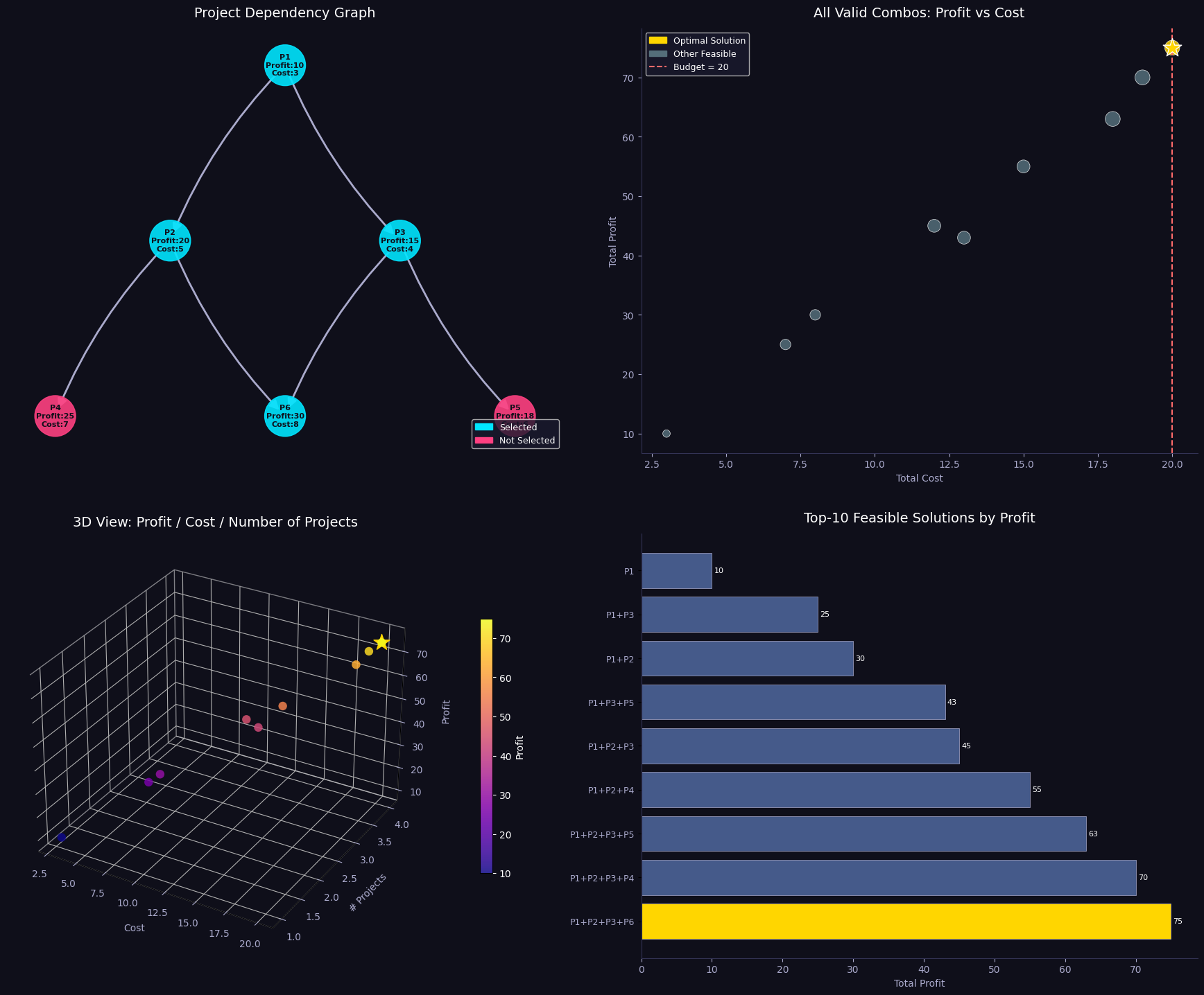
Chart saved as project_selection.png
Interpretation of Results
The ILP solver finds the globally optimal solution in microseconds, and the brute-force confirms it by checking all 64 subsets.
Key insights from the charts:
- Dependency chains dominate the structure. P6 (profit 30) requires both P2 and P3, which in turn both require P1. Selecting P6 alone consumes a minimum of $3 + 5 + 4 + 8 = 20$ units — the entire budget.
- The 3D plot exposes a Pareto-like frontier: portfolios that spend close to the budget tend to achieve higher profits, but only when the dependency graph is respected.
- Expensive does not mean profitable. Some three-project combos yield less profit than two-project combos because prerequisite projects add cost without contributing much profit directly.
This example clearly demonstrates why greedy heuristics fail on dependency-constrained problems — and why Integer Linear Programming is the right tool for the job.