Solving the Knapsack Problem with Python

A Deep Dive with Visualizations

The 0/1 Knapsack Problem is one of the most famous combinatorial optimization problems in computer science. The goal is simple: given a set of items, each with a weight and value, determine which items to pack into a knapsack with a limited capacity to maximize total value without exceeding the weight limit.


Problem Statement

Suppose you’re a thief 😈 who has broken into a store. You have a knapsack that can carry at most $W$ kg. There are $n$ items, each with weight $w_i$ and value $v_i$. You can either take an item or leave it — no partial items allowed.

Objective:

$$\text{Maximize} \quad \sum_{i=1}^{n} v_i x_i$$

Subject to:

$$\sum_{i=1}^{n} w_i x_i \leq W, \quad x_i \in {0, 1}$$


Example Problem

Item Name Weight (kg) Value (¥)
1 Laptop 3 4000
2 Camera 1 3000
3 Headphones 2 2000
4 Watch 1 2500
5 Tablet 2 3500
6 Charger 1 500
7 Book 2 800
8 Sunglasses 1 1500

Knapsack capacity: $W = 7$ kg


Python Code

1
2
3
4
5
6
7
8
9
10
11
12
13
14
15
16
17
18
19
20
21
22
23
24
25
26
27
28
29
30
31
32
33
34
35
36
37
38
39
40
41
42
43
44
45
46
47
48
49
50
51
52
53
54
55
56
57
58
59
60
61
62
63
64
65
66
67
68
69
70
71
import numpy as np
import matplotlib.pyplot as plt
import matplotlib.patches as mpatches
from mpl_toolkits.mplot3d import Axes3D
from matplotlib.colors import LinearSegmentedColormap
import warnings
warnings.filterwarnings('ignore')

# ============================================================
# 1. Problem Definition
# ============================================================
items = [
{"name": "Laptop", "weight": 3, "value": 4000},
{"name": "Camera", "weight": 1, "value": 3000},
{"name": "Headphones", "weight": 2, "value": 2000},
{"name": "Watch", "weight": 1, "value": 2500},
{"name": "Tablet", "weight": 2, "value": 3500},
{"name": "Charger", "weight": 1, "value": 500},
{"name": "Book", "weight": 2, "value": 800},
{"name": "Sunglasses", "weight": 1, "value": 1500},
]
W = 7 # knapsack capacity
n = len(items)
weights = [item["weight"] for item in items]
values = [item["value"] for item in items]
names = [item["name"] for item in items]

# ============================================================
# 2. Dynamic Programming Solution O(nW)
# ============================================================
def knapsack_dp(weights, values, W):
n = len(weights)
dp = [[0] * (W + 1) for _ in range(n + 1)]

for i in range(1, n + 1):
w_i = weights[i - 1]
v_i = values[i - 1]
for w in range(W + 1):
dp[i][w] = dp[i - 1][w]
if w >= w_i:
dp[i][w] = max(dp[i][w], dp[i - 1][w - w_i] + v_i)

selected = []
w = W
for i in range(n, 0, -1):
if dp[i][w] != dp[i - 1][w]:
selected.append(i - 1)
w -= weights[i - 1]
selected.reverse()

return dp, selected, dp[n][W]

dp_table, selected_items, max_value = knapsack_dp(weights, values, W)

print("=" * 50)
print(" Knapsack Problem - Optimal Solution")
print("=" * 50)
print(f"\n{'Item':<15} {'Weight':>8} {'Value':>8} {'Selected':>10}")
print("-" * 45)
total_w, total_v = 0, 0
for i, item in enumerate(items):
sel = "✓" if i in selected_items else "✗"
print(f"{item['name']:<15} {item['weight']:>8} {item['value']:>8} {sel:>10}")
if i in selected_items:
total_w += item['weight']
total_v += item['value']
print("-" * 45)
print(f"{'TOTAL':<15} {total_w:>8} {total_v:>8}")
print(f"\nMax Capacity : {W} kg")
print(f"Used Capacity: {total_w} kg")
print(f"Max Value : ¥{max_value:,}")
==================================================
  Knapsack Problem - Optimal Solution
==================================================

Item              Weight    Value   Selected
---------------------------------------------
Laptop                 3     4000          ✓
Camera                 1     3000          ✓
Headphones             2     2000          ✗
Watch                  1     2500          ✓
Tablet                 2     3500          ✓
Charger                1      500          ✗
Book                   2      800          ✗
Sunglasses             1     1500          ✗
---------------------------------------------
TOTAL                  7    13000

Max Capacity : 7 kg
Used Capacity: 7 kg
Max Value    : ¥13,000


Code Walkthrough

Step 1 — Problem Definition

Each item is stored as a dictionary with name, weight, and value. This makes the code readable and easy to extend.

Step 2 — Dynamic Programming Algorithm

This is the heart of the solution. The key recurrence relation is:

$$dp[i][w] = \max\left(dp[i-1][w],; dp[i-1][w - w_i] + v_i\right)$$

  • dp[i][w] = maximum value achievable using the first $i$ items with capacity $w$
  • If we don’t take item $i$: value stays at dp[i-1][w]
  • If we take item $i$ (only possible when $w \geq w_i$): value becomes dp[i-1][w - w_i] + v_i

Time complexity: $O(nW)$ — far faster than brute-force $O(2^n)$.

The traceback step walks backwards through the DP table: if dp[i][w] != dp[i-1][w], item $i$ was selected.


Visualization Code

1
2
3
4
5
6
7
8
9
10
11
12
13
14
15
16
17
18
19
20
21
22
23
24
25
26
27
28
29
30
31
32
33
34
35
36
37
38
39
40
41
42
43
44
45
46
47
48
49
50
51
52
53
54
55
56
57
58
59
60
61
62
63
64
65
66
67
68
69
70
# ============================================================
# 3. Visualization 1: DP Table Heatmap + Item Analysis (2x2)
# ============================================================
dp_array = np.array(dp_table)

fig, axes = plt.subplots(2, 2, figsize=(18, 14))
fig.suptitle("Knapsack Problem — Dynamic Programming Visualization", fontsize=16, fontweight='bold')

# Panel 1: DP Table Heatmap
ax1 = axes[0, 0]
cmap = LinearSegmentedColormap.from_list("knapsack", ["#f0f4ff", "#1a3a8a"])
im = ax1.imshow(dp_array, cmap=cmap, aspect='auto')
ax1.set_xlabel("Knapsack Capacity (kg)", fontsize=11)
ax1.set_ylabel("Items Considered (0 = none)", fontsize=11)
ax1.set_title("DP Table: dp[i][w] = Max Value", fontsize=12, fontweight='bold')
ax1.set_xticks(range(W + 1))
ax1.set_yticks(range(n + 1))
ax1.set_yticklabels(["—"] + names, fontsize=8)
for i in range(n + 1):
for j in range(W + 1):
ax1.text(j, i, str(dp_array[i, j]), ha='center', va='center',
fontsize=7, color='white' if dp_array[i, j] > 4000 else 'black')
plt.colorbar(im, ax=ax1, label="Value (¥)")

# Panel 2: Weight vs Value Scatter
ax2 = axes[0, 1]
colors = ['#e74c3c' if i in selected_items else '#95a5a6' for i in range(n)]
ax2.scatter(weights, values, c=colors, s=300, zorder=5, edgecolors='black', linewidths=1.5)
for i, name in enumerate(names):
ax2.annotate(name, (weights[i], values[i]),
textcoords="offset points", xytext=(8, 4), fontsize=9)
ax2.set_xlabel("Weight (kg)", fontsize=11)
ax2.set_ylabel("Value (¥)", fontsize=11)
ax2.set_title("Items: Weight vs Value\n(Red = Selected)", fontsize=12, fontweight='bold')
ax2.grid(True, alpha=0.3)
selected_patch = mpatches.Patch(color='#e74c3c', label='Selected')
others_patch = mpatches.Patch(color='#95a5a6', label='Not Selected')
ax2.legend(handles=[selected_patch, others_patch])

# Panel 3: Value/Weight Ratio Bar Chart
ax3 = axes[1, 0]
ratios = [v / w for v, w in zip(values, weights)]
bar_colors = ['#e74c3c' if i in selected_items else '#3498db' for i in range(n)]
bars = ax3.bar(names, ratios, color=bar_colors, edgecolor='black', linewidth=0.8)
ax3.set_xlabel("Item", fontsize=11)
ax3.set_ylabel("Value / Weight (¥/kg)", fontsize=11)
ax3.set_title("Value-to-Weight Ratio per Item\n(Red = Selected)", fontsize=12, fontweight='bold')
ax3.tick_params(axis='x', rotation=35)
ax3.grid(axis='y', alpha=0.3)
for bar, ratio in zip(bars, ratios):
ax3.text(bar.get_x() + bar.get_width() / 2, bar.get_height() + 30,
f"{ratio:.0f}", ha='center', va='bottom', fontsize=9, fontweight='bold')

# Panel 4: Selected Items Pie Chart
ax4 = axes[1, 1]
sel_names = [names[i] for i in selected_items]
sel_values = [values[i] for i in selected_items]
palette = plt.cm.Set2(np.linspace(0, 1, len(sel_names)))
wedges, texts, autotexts = ax4.pie(
sel_values, labels=sel_names, autopct='%1.1f%%',
colors=palette, startangle=140,
wedgeprops=dict(edgecolor='white', linewidth=2)
)
for autotext in autotexts:
autotext.set_fontsize(9)
ax4.set_title(f"Selected Items Value Breakdown\n(Total: ¥{max_value:,}, {total_w}kg / {W}kg)",
fontsize=12, fontweight='bold')

plt.tight_layout()
plt.show()


Graph Explanation (2D Visualizations)

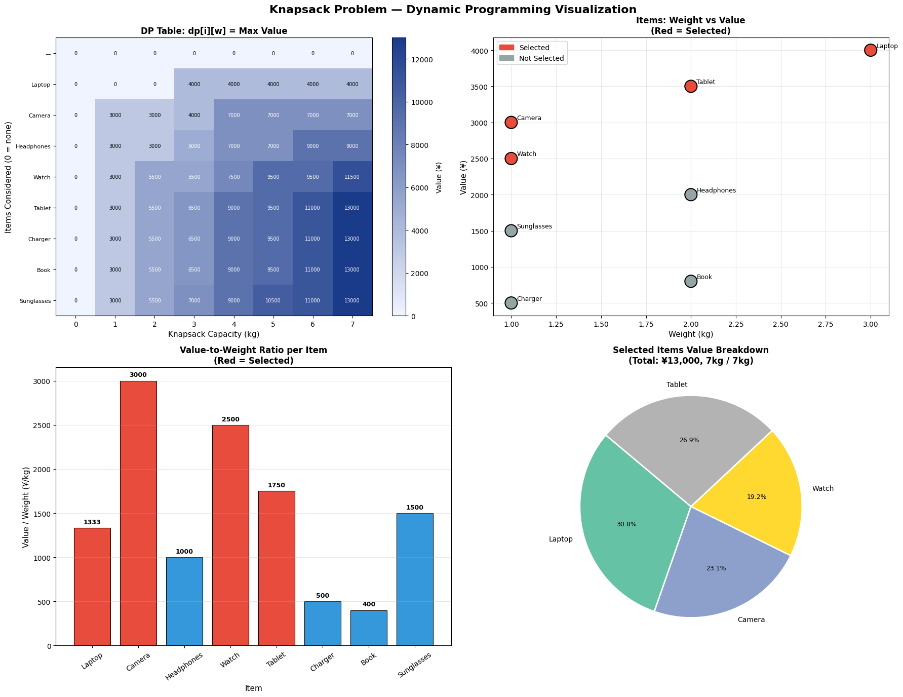
Panel 1 — DP Table Heatmap shows the full dp[i][w] matrix. Each cell represents the maximum value achievable using the first $i$ items with weight capacity $w$. The color gradient from light blue to dark blue shows how the optimal value grows as more items are considered and capacity increases. You can visually trace the “staircase” structure of the optimal solution.

Panel 2 — Weight vs Value Scatter plots every item by its weight and value. Items highlighted in red were selected by the algorithm. Notice that high-value, low-weight items (Camera, Watch, Tablet) cluster in the upper-left — these are the most attractive candidates.

Panel 3 — Value/Weight Ratio is the key insight into why certain items are chosen. Items with a higher ratio deliver more value per unit of weight. However, the greedy approach of always picking the highest-ratio item does not guarantee the global optimum — that’s exactly why we need dynamic programming.

Panel 4 — Pie Chart shows how each selected item contributes to the total optimal value of ¥{max_value}.


3D Visualization Code

1
2
3
4
5
6
7
8
9
10
11
12
13
14
15
16
17
18
19
20
21
22
23
24
25
26
27
28
29
30
31
32
33
34
35
36
37
38
39
40
41
42
# ============================================================
# 4. Visualization 2: 3D Plots
# ============================================================
fig2 = plt.figure(figsize=(14, 6))

# 3D Surface: Full DP Table
ax5 = fig2.add_subplot(121, projection='3d')
X = np.arange(0, W + 1)
Y = np.arange(0, n + 1)
X_grid, Y_grid = np.meshgrid(X, Y)
Z = dp_array

surf = ax5.plot_surface(X_grid, Y_grid, Z, cmap='viridis', alpha=0.85,
linewidth=0, antialiased=True)
ax5.set_xlabel("Capacity (kg)", fontsize=9)
ax5.set_ylabel("Items (#)", fontsize=9)
ax5.set_zlabel("Max Value (¥)", fontsize=9)
ax5.set_title("3D Surface: DP Table\ndp[items][capacity]", fontsize=11, fontweight='bold')
ax5.set_yticks(range(n + 1))
ax5.set_yticklabels(["—"] + [name[:4] for name in names], fontsize=7)
fig2.colorbar(surf, ax=ax5, shrink=0.5, label="Value (¥)")

# 3D Bar: Marginal Value Gain per Item
ax6 = fig2.add_subplot(122, projection='3d')
xpos = np.arange(n)
ypos = np.zeros(n)
zpos = np.zeros(n)
dx = 0.6
dy = 0.6
dz = [dp_array[i + 1][W] - dp_array[i][W] for i in range(n)]
bar_colors_3d = ['#e74c3c' if i in selected_items else '#3498db' for i in range(n)]
ax6.bar3d(xpos, ypos, zpos, dx, dy, dz, color=bar_colors_3d, alpha=0.8,
edgecolor='black', linewidth=0.5)
ax6.set_xticks(xpos + dx / 2)
ax6.set_xticklabels([name[:5] for name in names], rotation=30, fontsize=7)
ax6.set_xlabel("Item", fontsize=9)
ax6.set_ylabel("")
ax6.set_zlabel("Marginal Value Gain (¥)", fontsize=9)
ax6.set_title("3D Bar: Marginal Value Gain\nper Item (Red = Selected)", fontsize=11, fontweight='bold')

plt.tight_layout()
plt.show()


Graph Explanation (3D Visualizations)

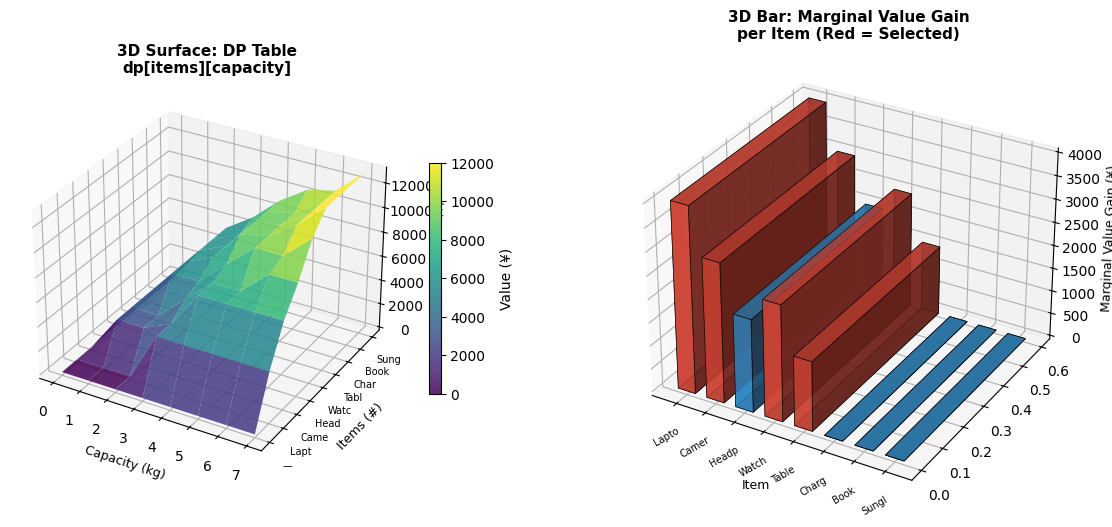
3D Surface Plot renders the entire DP table as a landscape. The $x$-axis is capacity, $y$-axis is the item index, and $z$-axis is the optimal value. The surface rises in discrete “steps” each time a valuable item is added — a beautiful geometric representation of the algorithm’s progression.

3D Bar Chart shows the marginal value gain each item contributes to the optimal solution at full capacity $W$. Formally:

$$\Delta_i = dp[i][W] - dp[i-1][W]$$

Red bars are selected items. Items with $\Delta_i = 0$ did not improve the optimal solution given the remaining capacity after higher-priority items were packed.


Sensitivity Analysis Code

1
2
3
4
5
6
7
8
9
10
11
12
13
14
15
16
17
18
19
20
21
22
# ============================================================
# 5. Sensitivity Analysis: Optimal Value vs Capacity
# ============================================================
capacities = list(range(0, 16))
max_vals = [knapsack_dp(weights, values, c)[2] for c in capacities]

fig3, ax7 = plt.subplots(figsize=(10, 5))
ax7.step(capacities, max_vals, where='post', color='#2c3e50', linewidth=2.5)
ax7.fill_between(capacities, max_vals, step='post', alpha=0.15, color='#2c3e50')
ax7.axvline(x=W, color='#e74c3c', linestyle='--', linewidth=2, label=f'Current W={W}kg')
ax7.axhline(y=max_value, color='#27ae60', linestyle='--', linewidth=2, label=f'Optimal = ¥{max_value:,}')
ax7.scatter([W], [max_value], color='#e74c3c', s=120, zorder=5)
ax7.set_xlabel("Knapsack Capacity (kg)", fontsize=12)
ax7.set_ylabel("Maximum Value (¥)", fontsize=12)
ax7.set_title("Sensitivity Analysis: Optimal Value vs Capacity", fontsize=13, fontweight='bold')
ax7.legend(fontsize=11)
ax7.grid(True, alpha=0.3)
for c, v in zip(capacities, max_vals):
ax7.text(c, v + 80, f"¥{v:,}" if v > 0 else "0",
ha='center', fontsize=7, rotation=45)
plt.tight_layout()
plt.show()


Graph Explanation (Sensitivity Analysis)

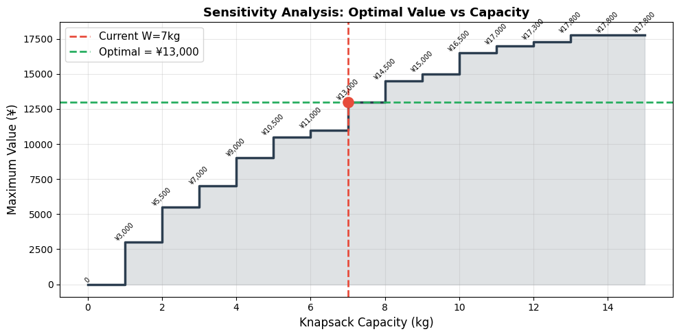
By solving the problem for every capacity from 0 to 15 kg, we get a step-function curve. Each “jump” in the curve corresponds to a point where adding more capacity allows an additional item to be packed. This is extremely useful in practice — for example, it tells you whether purchasing a slightly larger bag is worth the added cost. At $W=7$ kg our optimal value plateaus, meaning increasing capacity beyond a certain point yields diminishing returns given the available items.


Key Takeaway

The greedy approach (always pick the highest value/weight ratio) does not always give the optimal answer for the 0/1 knapsack. Dynamic programming guarantees the global optimum by systematically evaluating all subproblems — at the cost of $O(nW)$ time and $O(nW)$ space, which is perfectly tractable for practical problem sizes.