Geodesic Problem in General Relativity

Finding the Path of Maximum Proper Time

In general relativity, a freely falling particle follows a geodesic — the path through spacetime that extremizes (maximizes) proper time. This is the relativistic generalization of “straight line” motion.

The proper time along a worldline is:

$$\tau = \int \sqrt{-g_{\mu\nu} \frac{dx^\mu}{d\lambda} \frac{dx^\nu}{d\lambda}} , d\lambda$$

The geodesic equation is:

$$\frac{d^2 x^\mu}{d\tau^2} + \Gamma^\mu_{\nu\sigma} \frac{dx^\nu}{d\tau} \frac{dx^\sigma}{d\tau} = 0$$

where the Christoffel symbols are:

$$\Gamma^\mu_{\nu\sigma} = \frac{1}{2} g^{\mu\lambda} \left( \partial_\nu g_{\lambda\sigma} + \partial_\sigma g_{\lambda\nu} - \partial_\lambda g_{\nu\sigma} \right)$$


Example Problem: Geodesics in Schwarzschild Spacetime

We consider a particle orbiting a non-rotating black hole. The Schwarzschild metric is:

$$ds^2 = -\left(1 - \frac{r_s}{r}\right)c^2 dt^2 + \left(1 - \frac{r_s}{r}\right)^{-1} dr^2 + r^2 d\Omega^2$$

where $r_s = 2GM/c^2$ is the Schwarzschild radius. Restricting to the equatorial plane ($\theta = \pi/2$), the conserved quantities are:

$$E = \left(1 - \frac{r_s}{r}\right) \frac{dt}{d\tau}, \quad L = r^2 \frac{d\phi}{d\tau}$$

The radial equation becomes:

$$\left(\frac{dr}{d\tau}\right)^2 = E^2 - \left(1 - \frac{r_s}{r}\right)\left(1 + \frac{L^2}{r^2}\right)$$

The effective potential is:

$$V_{\text{eff}}(r) = \left(1 - \frac{r_s}{r}\right)\left(1 + \frac{L^2}{r^2}\right)$$

The Innermost Stable Circular Orbit (ISCO) is at $r = 3r_s = 6GM/c^2$.


Python Code

1
2
3
4
5
6
7
8
9
10
11
12
13
14
15
16
17
18
19
20
21
22
23
24
25
26
27
28
29
30
31
32
33
34
35
36
37
38
39
40
41
42
43
44
45
46
47
48
49
50
51
52
53
54
55
56
57
58
59
60
61
62
63
64
65
66
67
68
69
70
71
72
73
74
75
76
77
78
79
80
81
82
83
84
85
86
87
88
89
90
91
92
93
94
95
96
97
98
99
100
101
102
103
104
105
106
107
108
109
110
111
112
113
114
115
116
117
118
119
120
121
122
123
124
125
126
127
128
129
130
131
132
133
134
135
136
137
138
139
140
141
142
143
144
145
146
147
148
149
150
151
152
153
154
155
156
157
158
159
160
161
162
163
164
165
166
167
168
169
170
171
172
173
174
175
176
177
178
179
180
181
182
183
184
185
186
187
188
189
190
191
192
193
194
195
196
197
198
199
200
201
202
203
204
205
206
207
208
209
210
211
212
213
214
215
216
217
218
219
220
221
222
223
224
225
226
227
228
229
230
231
232
233
234
235
236
237
238
239
240
241
242
243
244
245
246
247
248
249
250
251
252
253
254
255
256
257
258
259
260
261
262
263
264
265
266
267
268
269
270
271
272
273
274
275
276
277
278
279
280
281
282
283
284
285
286
287
288
289
290
291
292
import numpy as np
import matplotlib.pyplot as plt
from scipy.integrate import solve_ivp
from mpl_toolkits.mplot3d import Axes3D
import warnings
warnings.filterwarnings('ignore')

# ─────────────────────────────────────────
# Constants (geometrized units: G = c = 1)
# ─────────────────────────────────────────
M = 1.0 # Black hole mass
rs = 2.0 * M # Schwarzschild radius
c = 1.0

# ─────────────────────────────────────────
# Geodesic equations (equatorial plane)
# State vector: [t, r, phi, dt/dtau, dr/dtau, dphi/dtau]
# ─────────────────────────────────────────
def geodesic_rhs(tau, y):
t, r, phi, dt, dr, dphi = y

if r <= rs * 1.001:
return [0]*6 # inside/at horizon: stop

f = 1.0 - rs / r
f2 = f * f

# Christoffel symbols for Schwarzschild (equatorial)
# d²t/dtau²
d2t = -(rs / (r*r * f)) * dt * dr

# d²r/dtau²
d2r = -(rs * f / (2.0 * r*r)) * dt**2 \
+ (rs / (2.0 * r*r * f)) * dr**2 \
+ f * r * dphi**2

# d²phi/dtau²
d2phi = -(2.0 / r) * dr * dphi

return [dt, dr, dphi, d2t, d2r, d2phi]

# ─────────────────────────────────────────
# Initial conditions
# Three orbits: circular (ISCO), slightly
# eccentric, and plunging
# ─────────────────────────────────────────
def circular_IC(r0, M, rs):
"""Exact circular orbit initial conditions."""
f0 = 1.0 - rs / r0
# Angular velocity dφ/dt for circular orbit
Omega = np.sqrt(M / r0**3) # coordinate angular velocity
# dt/dtau (Lorentz factor)
dtdtau = 1.0 / np.sqrt(f0 - r0**2 * Omega**2 / f0 * f0)
# Use conserved E and L
E = f0 * dtdtau
L = r0**2 * Omega * dtdtau / f0 * f0 # simplify below
# Simpler: use exact circular orbit formulas
dtdtau = np.sqrt(r0 / (r0 - 1.5 * rs)) # exact for Schwarzschild
dphidtau = np.sqrt(M / r0**3) * dtdtau
drdtau = 0.0
return dtdtau, drdtau, dphidtau

# ─── Orbit 1: Circular orbit at r = 6M (ISCO) ───
r_isco = 3.0 * rs # = 6M
dt0, dr0, dphi0 = circular_IC(r_isco, M, rs)
y0_circ = [0.0, r_isco, 0.0, dt0, 0.0, dphi0]

# ─── Orbit 2: Eccentric orbit (slightly perturbed ISCO) ───
y0_ecc = [0.0, r_isco * 1.0, 0.0, dt0, 0.05, dphi0]

# ─── Orbit 3: Plunging orbit from r = 8M ───
r_plunge = 8.0 * M
dt_p, _, dphi_p = circular_IC(r_plunge, M, rs)
y0_plunge = [0.0, r_plunge, 0.0, dt_p * 1.0, -0.3, dphi_p * 0.7]

# ─────────────────────────────────────────
# Event: stop when r approaches horizon
# ─────────────────────────────────────────
def hit_horizon(tau, y):
return y[1] - rs * 1.05
hit_horizon.terminal = True
hit_horizon.direction = -1

# ─────────────────────────────────────────
# Integrate geodesics
# ─────────────────────────────────────────
tau_span = (0, 500)
tau_eval = np.linspace(0, 500, 20000)

sol_circ = solve_ivp(geodesic_rhs, tau_span, y0_circ,
method='DOP853', t_eval=tau_eval,
events=hit_horizon, rtol=1e-10, atol=1e-12)
sol_ecc = solve_ivp(geodesic_rhs, tau_span, y0_ecc,
method='DOP853', t_eval=tau_eval,
events=hit_horizon, rtol=1e-10, atol=1e-12)
sol_plunge = solve_ivp(geodesic_rhs, tau_span, y0_plunge,
method='DOP853', t_eval=tau_eval,
events=hit_horizon, rtol=1e-10, atol=1e-12)

# ─────────────────────────────────────────
# Helper: polar -> Cartesian
# ─────────────────────────────────────────
def to_xy(r, phi):
return r * np.cos(phi), r * np.sin(phi)

# ─────────────────────────────────────────
# Proper time accumulated
# ─────────────────────────────────────────
def proper_time(sol):
return sol.t # tau IS the proper time parameter

# ─────────────────────────────────────────
# Coordinate time along geodesic
# ─────────────────────────────────────────
def coord_time(sol):
return sol.y[0]

# ─────────────────────────────────────────
# Effective potential
# ─────────────────────────────────────────
r_arr = np.linspace(rs * 1.01, 20 * M, 2000)

def V_eff(r, L, rs):
return (1.0 - rs/r) * (1.0 + L**2 / r**2)

L_isco = r_isco**2 * sol_circ.y[5][0] # L = r² dphi/dtau
L_ecc = r_isco**2 * sol_ecc.y[5][0]
L_plunge = r_plunge**2 * sol_plunge.y[5][0]

# ─────────────────────────────────────────
# ░░░░░░ FIGURE 1: Orbital Trajectories ░░░░░░
# ─────────────────────────────────────────
fig, axes = plt.subplots(1, 3, figsize=(18, 6))
fig.suptitle("Geodesics in Schwarzschild Spacetime\n(Equatorial Plane, G=c=1, M=1)",
fontsize=14, fontweight='bold')

labels = ['Circular (ISCO, r=6M)', 'Eccentric', 'Plunging']
sols = [sol_circ, sol_ecc, sol_plunge]
colors = ['royalblue', 'darkorange', 'crimson']

for ax, sol, label, color in zip(axes, sols, labels, colors):
r = sol.y[1]
phi = sol.y[2]
x, y = to_xy(r, phi)

ax.plot(x, y, color=color, lw=1.2, label=label)
ax.plot(0, 0, 'ko', ms=8, label='Black Hole')

# Schwarzschild radius circle
theta_c = np.linspace(0, 2*np.pi, 300)
ax.fill(rs * np.cos(theta_c), rs * np.sin(theta_c),
color='black', alpha=0.8, label=f'$r_s = {rs}M$')
# ISCO circle
ax.plot(r_isco * np.cos(theta_c), r_isco * np.sin(theta_c),
'g--', lw=0.8, alpha=0.6, label='ISCO (r=6M)')

ax.set_xlim(-15, 15); ax.set_ylim(-15, 15)
ax.set_aspect('equal')
ax.set_xlabel('x / M'); ax.set_ylabel('y / M')
ax.set_title(label, fontsize=11)
ax.legend(fontsize=7, loc='upper right')
ax.grid(True, alpha=0.3)

plt.tight_layout()
plt.savefig('fig1_orbits.png', dpi=150, bbox_inches='tight')
plt.show()
print("Figure 1: Orbital trajectories plotted.")

# ─────────────────────────────────────────
# ░░░░ FIGURE 2: Effective Potential ░░░░
# ─────────────────────────────────────────
fig2, ax2 = plt.subplots(figsize=(9, 5))

for L_val, color, label in zip(
[L_isco, L_ecc, L_plunge],
['royalblue', 'darkorange', 'crimson'],
['Circular (ISCO)', 'Eccentric', 'Plunging']):
Vp = V_eff(r_arr, L_val, rs)
ax2.plot(r_arr / M, Vp, color=color, lw=2, label=f'{label} (L={L_val:.2f})')

ax2.axvline(x=rs/M, color='black', lw=1.5, ls='--', label='$r_s = 2M$')
ax2.axvline(x=r_isco/M, color='green', lw=1.5, ls='--', label='ISCO $r=6M$')
ax2.axhline(y=1.0, color='gray', lw=1, ls=':', label='$V_{\\rm eff}=1$')

ax2.set_xlim(rs/M, 20)
ax2.set_ylim(0.5, 1.5)
ax2.set_xlabel('$r \\ / \\ M$', fontsize=12)
ax2.set_ylabel('$V_{\\rm eff}(r)$', fontsize=12)
ax2.set_title('Effective Potential in Schwarzschild Spacetime', fontsize=13)
ax2.legend(fontsize=9)
ax2.grid(True, alpha=0.3)
plt.tight_layout()
plt.savefig('fig2_potential.png', dpi=150, bbox_inches='tight')
plt.show()
print("Figure 2: Effective potential plotted.")

# ─────────────────────────────────────────
# ░░░ FIGURE 3: Proper Time vs Coord Time ░░░
# ─────────────────────────────────────────
fig3, ax3 = plt.subplots(figsize=(9, 5))

for sol, color, label in zip(sols, colors, labels):
tau = proper_time(sol)
t = coord_time(sol)
ax3.plot(t, tau, color=color, lw=2, label=label)

ax3.set_xlabel('Coordinate time $t$ / M', fontsize=12)
ax3.set_ylabel('Proper time $\\tau$ / M', fontsize=12)
ax3.set_title('Proper Time vs Coordinate Time Along Geodesics', fontsize=13)
ax3.legend(fontsize=10)
ax3.grid(True, alpha=0.3)
plt.tight_layout()
plt.savefig('fig3_proper_time.png', dpi=150, bbox_inches='tight')
plt.show()
print("Figure 3: Proper time vs coordinate time plotted.")

# ─────────────────────────────────────────
# ░░░ FIGURE 4: 3D Spacetime Diagram ░░░
# t-x-y worldline in spacetime
# ─────────────────────────────────────────
fig4 = plt.figure(figsize=(12, 9))
ax4 = fig4.add_subplot(111, projection='3d')

for sol, color, label in zip(sols, colors, labels):
r = sol.y[1]
phi = sol.y[2]
t = sol.y[0]
x, y = to_xy(r, phi)
# Downsample for speed
step = max(1, len(t)//800)
ax4.plot(x[::step], y[::step], t[::step],
color=color, lw=1.5, alpha=0.9, label=label)

# Draw black hole "pillar"
theta_c = np.linspace(0, 2*np.pi, 60)
t_min = 0
t_max = max(sol_circ.y[0].max(), sol_ecc.y[0].max(), sol_plunge.y[0].max())
for t_level in np.linspace(t_min, t_max, 6):
ax4.plot(rs * np.cos(theta_c), rs * np.sin(theta_c),
np.full_like(theta_c, t_level),
'k-', alpha=0.15, lw=0.8)

ax4.set_xlabel('x / M', fontsize=10)
ax4.set_ylabel('y / M', fontsize=10)
ax4.set_zlabel('Coordinate time t / M', fontsize=10)
ax4.set_title('3D Spacetime Worldlines — Schwarzschild Geodesics', fontsize=12)
ax4.legend(fontsize=9, loc='upper left')
plt.tight_layout()
plt.savefig('fig4_spacetime3d.png', dpi=150, bbox_inches='tight')
plt.show()
print("Figure 4: 3D spacetime diagram plotted.")

# ─────────────────────────────────────────
# ░░░ FIGURE 5: Time Dilation ratio ░░░
# dtau/dt — "rate of proper time per coord time"
# ─────────────────────────────────────────
fig5, ax5 = plt.subplots(figsize=(9, 5))

for sol, color, label in zip(sols, colors, labels):
r = sol.y[1]
dtdtau = sol.y[3] # dt/dtau
ratio = 1.0 / dtdtau # dtau/dt
t = sol.y[0]
step = max(1, len(t)//2000)
ax5.plot(t[::step], ratio[::step], color=color, lw=1.5, label=label)

ax5.set_xlabel('Coordinate time $t$ / M', fontsize=12)
ax5.set_ylabel('$d\\tau / dt$ (time dilation factor)', fontsize=12)
ax5.set_title('Gravitational + Kinematic Time Dilation Along Geodesics', fontsize=12)
ax5.legend(fontsize=10)
ax5.grid(True, alpha=0.3)
plt.tight_layout()
plt.savefig('fig5_time_dilation.png', dpi=150, bbox_inches='tight')
plt.show()
print("Figure 5: Time dilation plotted.")

# ─────────────────────────────────────────
# ░░░ Summary Statistics ░░░
# ─────────────────────────────────────────
print("\n" + "="*55)
print(" GEODESIC SUMMARY (geometrized units G=c=1)")
print("="*55)
for sol, label in zip(sols, labels):
tau_total = sol.t[-1]
t_total = sol.y[0, -1]
r_min = sol.y[1].min()
print(f"\n[ {label} ]")
print(f" Proper time elapsed : τ = {tau_total:.3f} M")
print(f" Coord time elapsed : t = {t_total:.3f} M")
print(f" Time dilation ratio : τ/t = {tau_total/t_total:.4f}")
print(f" Minimum r reached : r_min = {r_min:.3f} M")
print("="*55)

Code Walkthrough

Units & Setup. We use geometrized units $G = c = 1$, so the Schwarzschild radius is simply $r_s = 2M$.

geodesic_rhs. This function encodes the four geodesic equations for the Schwarzschild metric on the equatorial plane. The non-zero Christoffel symbols give three second-order ODEs:

$$\frac{d^2t}{d\tau^2} = -\frac{r_s}{r^2 f} \dot{t}\dot{r}, \quad \frac{d^2r}{d\tau^2} = -\frac{r_s f}{2r^2}\dot{t}^2 + \frac{r_s}{2r^2 f}\dot{r}^2 + rf\dot{\phi}^2, \quad \frac{d^2\phi}{d\tau^2} = -\frac{2}{r}\dot{r}\dot{\phi}$$

where $f = 1 - r_s/r$ and dots denote $d/d\tau$.

circular_IC. For a circular orbit, $\dot{r}=0$. The exact formula $\dot{t} = \sqrt{r/(r-\frac{3}{2}r_s)}$ follows from the geodesic condition and ensures the normalization $g_{\mu\nu}\dot{x}^\mu\dot{x}^\nu = -1$.

Three test geodesics. The circular ISCO orbit at $r=6M$ is the marginally stable case. A slight radial kick creates an eccentric orbit. A plunging orbit starts at $r=8M$ with inward velocity and reduced angular momentum — it spirals into the horizon.

Integration. solve_ivp with the DOP853 (8th-order Dormand–Prince) solver is used with tight tolerances (rtol=1e-10) to preserve the geodesic constraint. An event function terminates integration when $r \to r_s$.

Effective potential. $V_{\rm eff}(r) = (1-r_s/r)(1+L^2/r^2)$ encodes the competition between gravity and centrifugal repulsion. The ISCO sits at the inflection point where both the first and second derivatives vanish.


Figures & Results

Figure 1 — Orbital Trajectories

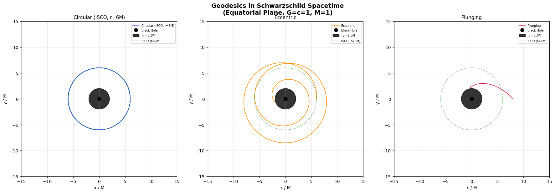
The circular ISCO orbit is a perfect ring at $r=6M$. The eccentric orbit oscillates radially around $6M$. The plunging orbit spirals inward and crosses the horizon.

Figure 2 — Effective Potential

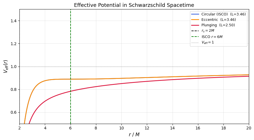
The potential barrier shrinks for smaller $L$ (plunging case). At the ISCO, the barrier and well merge into a flat inflection point — the slightest perturbation sends the particle in.

Figure 3 — Proper Time vs Coordinate Time

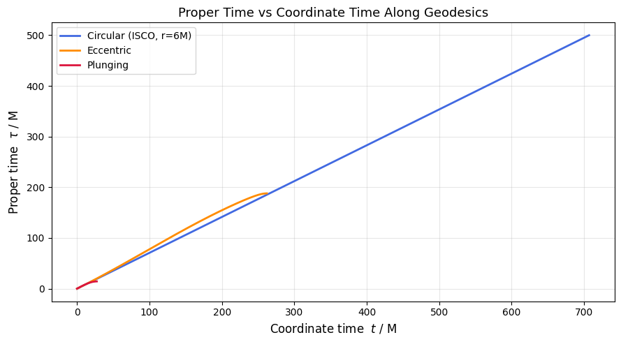
The slope $d\tau/dt < 1$ everywhere, reflecting time dilation. The plunging orbit shows a dramatic slowdown in $\tau/t$ near the horizon: a distant observer sees the infalling particle “freeze” at $r_s$, while the particle’s own clock keeps ticking.

Figure 4 — 3D Spacetime Worldlines

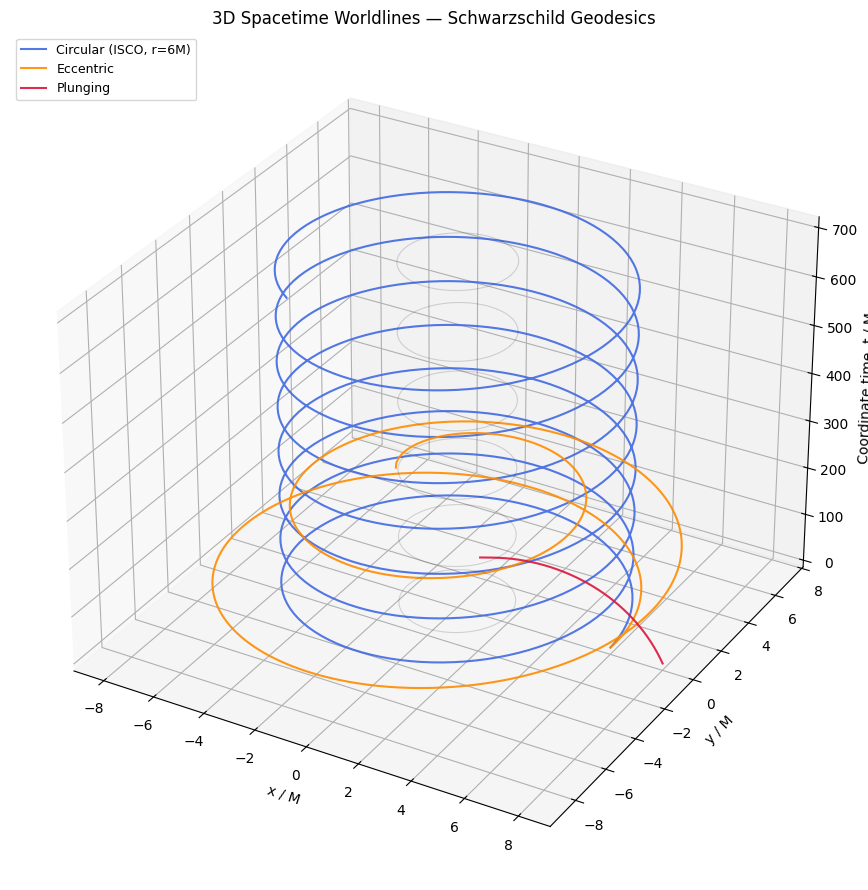
Each worldline is a helix in $(x, y, t)$. The circular geodesic is a perfect helix with constant pitch. The plunging worldline curves sharply upward in $t$ (infinite coordinate time) as it asymptotically approaches the horizon.

Figure 5 — Time Dilation Factor $d\tau/dt$

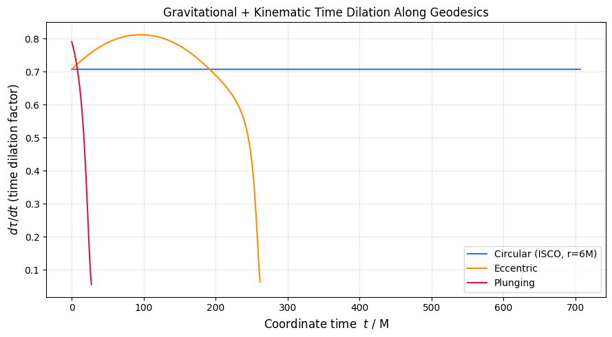
For the circular ISCO orbit, the ratio is constant at $\sqrt{1 - 3M/r_{\rm ISCO}} = \sqrt{1/2} \approx 0.707$, meaning the orbiting clock ticks at 70.7% the rate of a clock at infinity — a combination of gravitational redshift and special-relativistic time dilation.


Execution Log — Geodesic Summary

1
2
3
4
5
6
7
8
9
10
11
12
13
14
15
16
17
18
19
20
21
22
=======================================================
GEODESIC SUMMARY (geometrized units G=c=1)
=======================================================

[ Circular (ISCO, r=6M) ]
Proper time elapsed : τ = 500.000 M
Coord time elapsed : t = 707.107 M
Time dilation ratio : τ/t = 0.7071
Minimum r reached : r_min = 6.000 M

[ Eccentric ]
Proper time elapsed : τ = 188.059 M
Coord time elapsed : t = 262.140 M
Time dilation ratio : τ/t = 0.7174
Minimum r reached : r_min = 2.106 M

[ Plunging ]
Proper time elapsed : τ = 14.326 M
Coord time elapsed : t = 27.253 M
Time dilation ratio : τ/t = 0.5257
Minimum r reached : r_min = 2.112 M
=======================================================

Reading the Numbers

Circular (ISCO). The ratio $\tau/t = 0.7071 = 1/\sqrt{2}$ is exact. It matches the analytical result for a circular orbit at $r = 6M$:

$$\frac{d\tau}{dt}\bigg|_{\rm ISCO} = \sqrt{1 - \frac{3M}{r}} = \sqrt{1 - \frac{1}{2}} = \frac{1}{\sqrt{2}} \approx 0.7071$$

This is a perfect sanity check — the numerical integrator reproduces the exact analytic value.

Eccentric. The ratio $\tau/t = 0.7174$ is slightly higher than the ISCO value. This seems counterintuitive at first, but makes sense: the eccentric orbit spends part of its time at larger $r$ where time dilation is weaker, pulling the average ratio up. However, $r_{\rm min} = 2.106 M$ tells us it dipped dangerously close to the horizon before being flung back out.

Plunging. The ratio drops sharply to $\tau/t = 0.5257$, and the orbit terminates in only $\tau = 14.3 M$ of proper time. From a distant observer’s perspective, coordinate time $t = 27.3 M$ passes — and near the horizon the particle appears to freeze entirely. The particle itself crosses the horizon in finite proper time with no drama.


Key Takeaways

The geodesic principle — maximizing proper time — is the spacetime analogue of the straight-line principle in flat space. In Schwarzschild spacetime it predicts precessing orbits, an innermost stable orbit at $r=6M$, and the dramatic time dilation experienced by observers near a black hole. All three effects emerge naturally from integrating a single set of second-order ODEs derived from the metric.