Quantum Optimal Control

Shaping Laser Pulses to Drive Quantum State Transitions

Quantum control is one of the most fascinating intersections of physics and optimization theory. The central question is: can we design an external field (like a laser pulse) to steer a quantum system from one state to another with maximum fidelity? In this post, we tackle a concrete example using GRAPE (Gradient Ascent Pulse Engineering) — one of the most powerful algorithms in quantum optimal control.


The Problem

We consider a two-level quantum system (a qubit) with the Hamiltonian:

$$H(t) = H_0 + u(t) H_c$$

where:

$$H_0 = \frac{\omega_0}{2} \sigma_z, \quad H_c = \frac{\Omega}{2} \sigma_x$$

  • $H_0$ is the free (drift) Hamiltonian with transition frequency $\omega_0$
  • $H_c$ is the control Hamiltonian driven by laser amplitude $u(t)$
  • $\sigma_x, \sigma_z$ are Pauli matrices

Goal: Starting from $|\psi_0\rangle = |0\rangle$, find the optimal pulse $u(t)$ that drives the system to the target state $|\psi_{\text{target}}\rangle = |1\rangle$ (a population inversion, like a $\pi$-pulse) within time $T$.

The fidelity (objective to maximize) is:

$$\mathcal{F} = \left| \langle \psi_{\text{target}} | U(T) | \psi_0 \rangle \right|^2$$

where $U(T) = \mathcal{T} \exp\left( -i \int_0^T H(t) dt \right)$ is the time-evolution operator.


GRAPE Algorithm

We discretize time into $N$ steps of width $\Delta t = T/N$, so $u(t) \to {u_k}_{k=1}^N$. The propagator becomes:

$$U(T) = \prod_{k=N}^{1} e^{-i H_k \Delta t}, \quad H_k = H_0 + u_k H_c$$

The gradient of fidelity with respect to each control amplitude is:

$$\frac{\partial \mathcal{F}}{\partial u_k} = 2 \Delta t \cdot \text{Im}\left[ \langle \lambda_k | H_c | \phi_k \rangle \cdot \overline{\langle \psi_{\text{target}} | U(T) | \psi_0 \rangle} \right]$$

where $|\phi_k\rangle$ is the forward-propagated state and $|\lambda_k\rangle$ is the backward-propagated (co-state).


Python ImplementationHere’s the complete, tested Python code:

1
2
3
4
5
6
7
8
9
10
11
12
13
14
15
16
17
18
19
20
21
22
23
24
25
26
27
28
29
30
31
32
33
34
35
36
37
38
39
40
41
42
43
44
45
46
47
48
49
50
51
52
53
54
55
56
57
58
59
60
61
62
63
64
65
66
67
68
69
70
71
72
73
74
75
76
77
78
79
80
81
82
83
84
85
86
87
88
89
90
91
92
93
94
95
96
97
98
99
100
101
102
103
104
105
106
107
108
109
110
111
112
113
114
115
116
117
118
119
120
121
122
123
124
125
126
127
128
129
130
131
132
133
134
135
136
137
138
139
140
141
142
143
144
145
146
147
148
149
150
151
152
153
154
155
156
157
158
159
160
161
162
163
164
165
166
167
168
169
170
171
172
173
174
175
176
177
178
179
180
181
182
183
184
185
186
187
188
189
190
191
192
193
194
195
196
197
198
199
200
201
202
203
204
205
206
207
208
209
210
211
212
213
214
215
216
217
218
219
220
221
222
223
224
225
226
227
228
229
230
231
232
233
234
235
236
237
238
239
240
241
242
243
244
245
246
247
248
249
250
251
252
253
254
255
256
257
258
259
260
261
262
263
264
265
266
267
268
269
270
271
272
273
# ============================================================
# Quantum Optimal Control: GRAPE Algorithm for Qubit π-Pulse
# ============================================================

import numpy as np
import matplotlib.pyplot as plt
from mpl_toolkits.mplot3d import Axes3D
from scipy.linalg import expm
import warnings
warnings.filterwarnings('ignore')

# ─────────────────────────────────────────
# 1. System Parameters
# ─────────────────────────────────────────
omega0 = 2 * np.pi * 1.0 # transition frequency [rad/ns]
Omega = 2 * np.pi * 0.5 # max Rabi frequency [rad/ns]
T = 5.0 # total pulse duration [ns]
N = 100 # number of time steps
dt = T / N # time step size

# Pauli matrices
sx = np.array([[0, 1], [1, 0]], dtype=complex)
sy = np.array([[0, -1j], [1j, 0]], dtype=complex)
sz = np.array([[1, 0], [0, -1]], dtype=complex)

# Hamiltonians
H0 = (omega0 / 2) * sz # drift Hamiltonian
Hc = (Omega / 2) * sx # control Hamiltonian

# Initial and target states
psi0 = np.array([1, 0], dtype=complex) # |0⟩
psi_tgt = np.array([0, 1], dtype=complex) # |1⟩

# ─────────────────────────────────────────
# 2. Helper Functions
# ─────────────────────────────────────────
def propagator(u_k, dt):
"""Single-step propagator exp(-i H_k dt)."""
H_k = H0 + u_k * Hc
return expm(-1j * H_k * dt)

def forward_states(u_list):
"""Forward-propagate |psi0⟩ through all time steps.
Returns list of states BEFORE each step (length N+1)."""
states = [psi0.copy()]
for u_k in u_list:
U_k = propagator(u_k, dt)
states.append(U_k @ states[-1])
return states # states[k] = state at beginning of step k

def total_propagator(u_list):
"""Full time-evolution operator U(T)."""
U = np.eye(2, dtype=complex)
for u_k in reversed(u_list): # U_N...U_1
U = propagator(u_k, dt) @ U
return U

def fidelity(u_list):
"""F = |<psi_tgt|U(T)|psi0>|^2"""
U_T = total_propagator(u_list)
amp = psi_tgt.conj() @ (U_T @ psi0)
return np.abs(amp)**2

def grape_gradients(u_list):
"""Compute GRAPE gradients dF/du_k for all k."""
# Forward propagation
fwd = forward_states(u_list) # fwd[k] = phi_k

# Full propagator overlap
U_T = total_propagator(u_list)
overlap = psi_tgt.conj() @ (U_T @ psi0) # complex scalar

# Backward co-states: |lambda_k⟩ = U_{k+1}...U_N^† |psi_tgt⟩
# We propagate backward from target
co = psi_tgt.copy()
co_states = [None] * (N + 1)
co_states[N] = co.copy()
for k in range(N - 1, -1, -1):
U_k = propagator(u_list[k], dt)
co_states[k] = U_k.conj().T @ co_states[k + 1]

grads = np.zeros(N)
for k in range(N):
phi_k = fwd[k] # state before step k
lambda_k = co_states[k + 1] # co-state after step k
matrix_element = lambda_k.conj() @ ((-1j * Hc * dt) @ (propagator(u_list[k], dt) @ phi_k))
grads[k] = 2 * np.real(np.conj(overlap) * matrix_element)
return grads

# ─────────────────────────────────────────
# 3. GRAPE Optimization Loop
# ─────────────────────────────────────────
np.random.seed(42)
u = np.random.uniform(-0.3, 0.3, N) # random initial pulse

lr = 0.5 # learning rate
n_iter = 800 # number of iterations
u_max = 1.5 # amplitude clipping
fidelity_log = []
pulse_history = []

print("Starting GRAPE optimization...")
print(f"{'Iter':>6} | {'Fidelity':>10} | {'Max |u|':>10}")
print("-" * 35)

for i in range(n_iter):
F = fidelity(u)
fidelity_log.append(F)

if i % 100 == 0:
print(f"{i:>6} | {F:>10.6f} | {np.max(np.abs(u)):>10.4f}")

if F > 0.9999:
print(f"\n✓ Converged at iteration {i} with F = {F:.8f}")
break

grads = grape_gradients(u)
u = u + lr * grads
u = np.clip(u, -u_max, u_max) # enforce amplitude constraint

print(f"\nFinal fidelity: {fidelity(u):.8f}")

# ─────────────────────────────────────────
# 4. Bloch Sphere Trajectory
# ─────────────────────────────────────────
def bloch_vector(psi):
"""Compute Bloch vector (x,y,z) from state vector."""
rho = np.outer(psi, psi.conj())
return np.real(np.trace(sx @ rho)), np.real(np.trace(sy @ rho)), np.real(np.trace(sz @ rho))

fwd_states = forward_states(u)
bloch_traj = np.array([bloch_vector(s) for s in fwd_states])
bx, by, bz = bloch_traj[:, 0], bloch_traj[:, 1], bloch_traj[:, 2]

# ─────────────────────────────────────────
# 5. Visualization
# ─────────────────────────────────────────
fig = plt.figure(figsize=(18, 14))
fig.patch.set_facecolor('#0d0d0d')
cmap_pulse = plt.cm.plasma
cmap_traj = plt.cm.cool

t_arr = np.linspace(0, T, N)

# ── Panel 1: Optimized Pulse Shape ──────
ax1 = fig.add_subplot(2, 3, 1)
ax1.set_facecolor('#1a1a1a')
colors = cmap_pulse(np.linspace(0, 1, N))
for k in range(N - 1):
ax1.plot(t_arr[k:k+2], u[k:k+2], color=colors[k], lw=2)
ax1.axhline(0, color='gray', lw=0.8, ls='--')
ax1.fill_between(t_arr, u, alpha=0.2, color='#ff6ec7')
ax1.set_xlabel('Time (ns)', color='white')
ax1.set_ylabel('Amplitude u(t)', color='white')
ax1.set_title('Optimized Laser Pulse u(t)', color='white', fontsize=12, fontweight='bold')
ax1.tick_params(colors='white')
for spine in ax1.spines.values(): spine.set_color('#444')

# ── Panel 2: Fidelity Convergence ───────
ax2 = fig.add_subplot(2, 3, 2)
ax2.set_facecolor('#1a1a1a')
iters = np.arange(len(fidelity_log))
ax2.plot(iters, fidelity_log, color='#00ffcc', lw=2)
ax2.fill_between(iters, fidelity_log, alpha=0.15, color='#00ffcc')
ax2.axhline(1.0, color='#ff4444', ls='--', lw=1, label='F = 1')
ax2.set_xlabel('Iteration', color='white')
ax2.set_ylabel('Fidelity $\\mathcal{F}$', color='white')
ax2.set_title('GRAPE Convergence', color='white', fontsize=12, fontweight='bold')
ax2.legend(facecolor='#222', labelcolor='white')
ax2.tick_params(colors='white')
for spine in ax2.spines.values(): spine.set_color('#444')

# ── Panel 3: Population Dynamics ────────
ax3 = fig.add_subplot(2, 3, 3)
ax3.set_facecolor('#1a1a1a')
pop0 = np.array([np.abs(s[0])**2 for s in fwd_states])
pop1 = np.array([np.abs(s[1])**2 for s in fwd_states])
t_full = np.linspace(0, T, N + 1)
ax3.plot(t_full, pop0, color='#4fc3f7', lw=2, label='$P_{|0\\rangle}$')
ax3.plot(t_full, pop1, color='#ff6ec7', lw=2, label='$P_{|1\\rangle}$')
ax3.set_xlabel('Time (ns)', color='white')
ax3.set_ylabel('Population', color='white')
ax3.set_title('State Population Dynamics', color='white', fontsize=12, fontweight='bold')
ax3.legend(facecolor='#222', labelcolor='white')
ax3.tick_params(colors='white')
for spine in ax3.spines.values(): spine.set_color('#444')

# ── Panel 4: 3D Bloch Sphere ─────────────
ax4 = fig.add_subplot(2, 3, 4, projection='3d')
ax4.set_facecolor('#1a1a1a')
fig.patch.set_facecolor('#0d0d0d')

# Draw Bloch sphere wireframe
u_s = np.linspace(0, 2*np.pi, 30)
v_s = np.linspace(0, np.pi, 30)
xs = np.outer(np.cos(u_s), np.sin(v_s))
ys = np.outer(np.sin(u_s), np.sin(v_s))
zs = np.outer(np.ones(30), np.cos(v_s))
ax4.plot_wireframe(xs, ys, zs, color='#333333', lw=0.4, alpha=0.5)

# Axes
for vec, col, lbl in [([1,0,0],'#ff4444','x'), ([0,1,0],'#44ff44','y'), ([0,0,1],'#4444ff','z')]:
ax4.quiver(0,0,0,*vec, color=col, lw=1.5, arrow_length_ratio=0.1)
ax4.text(vec[0]*1.15, vec[1]*1.15, vec[2]*1.15, lbl, color=col, fontsize=10)

# Trajectory with color gradient
for k in range(len(bx)-1):
c = cmap_traj(k / len(bx))
ax4.plot(bx[k:k+2], by[k:k+2], bz[k:k+2], color=c, lw=2.5)

# Start and end markers
ax4.scatter(*bloch_vector(psi0), color='#00ff88', s=80, zorder=5, label='Start |0⟩')
ax4.scatter(*bloch_vector(psi_tgt), color='#ff6600', s=80, zorder=5, label='Target |1⟩')
ax4.scatter(bx[-1], by[-1], bz[-1], color='white', s=60, marker='*', zorder=6, label='Final state')

ax4.set_xlim(-1.2, 1.2); ax4.set_ylim(-1.2, 1.2); ax4.set_zlim(-1.2, 1.2)
ax4.set_xlabel('X', color='white'); ax4.set_ylabel('Y', color='white'); ax4.set_zlabel('Z', color='white')
ax4.set_title('Bloch Sphere Trajectory', color='white', fontsize=12, fontweight='bold')
ax4.tick_params(colors='white')
ax4.legend(facecolor='#222', labelcolor='white', fontsize=8, loc='upper left')

# ── Panel 5: Pulse Spectrum (FFT) ────────
ax5 = fig.add_subplot(2, 3, 5)
ax5.set_facecolor('#1a1a1a')
freqs = np.fft.rfftfreq(N, d=dt)
spectrum = np.abs(np.fft.rfft(u))**2
ax5.plot(freqs, spectrum, color='#ffcc00', lw=2)
ax5.fill_between(freqs, spectrum, alpha=0.2, color='#ffcc00')
ax5.axvline(omega0 / (2*np.pi), color='#ff4444', ls='--', lw=1.5, label=f'$\\omega_0/2\\pi$ = {omega0/(2*np.pi):.2f} GHz')
ax5.set_xlabel('Frequency (GHz)', color='white')
ax5.set_ylabel('Power Spectral Density', color='white')
ax5.set_title('Pulse Frequency Spectrum', color='white', fontsize=12, fontweight='bold')
ax5.legend(facecolor='#222', labelcolor='white')
ax5.tick_params(colors='white')
ax5.set_xlim(0, 3)
for spine in ax5.spines.values(): spine.set_color('#444')

# ── Panel 6: Bloch Vector Components ────
ax6 = fig.add_subplot(2, 3, 6)
ax6.set_facecolor('#1a1a1a')
ax6.plot(t_full, bx, color='#ff4444', lw=2, label='$\\langle\\sigma_x\\rangle$')
ax6.plot(t_full, by, color='#44ff44', lw=2, label='$\\langle\\sigma_y\\rangle$')
ax6.plot(t_full, bz, color='#4488ff', lw=2, label='$\\langle\\sigma_z\\rangle$')
ax6.axhline(0, color='gray', lw=0.5, ls='--')
ax6.set_xlabel('Time (ns)', color='white')
ax6.set_ylabel('Expectation Value', color='white')
ax6.set_title('Bloch Vector Components', color='white', fontsize=12, fontweight='bold')
ax6.legend(facecolor='#222', labelcolor='white')
ax6.tick_params(colors='white')
for spine in ax6.spines.values(): spine.set_color('#444')

plt.suptitle('Quantum Optimal Control — GRAPE Algorithm\n(Two-Level System π-Pulse)',
color='white', fontsize=14, fontweight='bold', y=1.01)
plt.tight_layout()
plt.savefig('quantum_control_grape.png', dpi=150, bbox_inches='tight',
facecolor='#0d0d0d')
plt.show()
print("\n[Figure saved as quantum_control_grape.png]")

# ─────────────────────────────────────────
# 6. Summary Statistics
# ─────────────────────────────────────────
final_state = fwd_states[-1]
print("\n══════════════════════════════════════")
print(" OPTIMIZATION SUMMARY ")
print("══════════════════════════════════════")
print(f" Final fidelity : {fidelity(u):.8f}")
print(f" Final state |0⟩ pop : {np.abs(final_state[0])**2:.6f}")
print(f" Final state |1⟩ pop : {np.abs(final_state[1])**2:.6f}")
print(f" Pulse RMS amplitude : {np.sqrt(np.mean(u**2)):.4f}")
print(f" Pulse peak amplitude : {np.max(np.abs(u)):.4f}")
print(f" Iterations run : {len(fidelity_log)}")
print("══════════════════════════════════════")

Code Walkthrough

Section 1 — System Parameters

We set up the physical parameters of our qubit. The drift Hamiltonian $H_0 = \frac{\omega_0}{2}\sigma_z$ governs the natural precession of the qubit around the $z$-axis at frequency $\omega_0 = 2\pi \times 1.0$ rad/ns. The control Hamiltonian $H_c = \frac{\Omega}{2}\sigma_x$ couples the laser field into the qubit via the $\sigma_x$ operator. We discretize the total evolution time $T = 5$ ns into $N = 100$ equal steps.

Section 2 — Helper Functions

propagator(u_k, dt) computes the matrix exponential $e^{-i H_k \Delta t}$ for a single time step using scipy.linalg.expm. This is the exact unitary evolution, no approximations. forward_states chains these propagators to give us the quantum state at every point in time. fidelity computes the overlap $|\langle\psi_\text{tgt}|U(T)|\psi_0\rangle|^2$.

Section 3 — GRAPE Gradient Computation

This is the algorithmic heart. At each step $k$, the GRAPE gradient is:

$$\frac{\partial \mathcal{F}}{\partial u_k} = 2,\text{Re}\left[\overline{\langle\psi_\text{tgt}|U(T)|\psi_0\rangle} \cdot \langle\lambda_{k+1}|(-i H_c \Delta t), U_k|\phi_k\rangle\right]$$

where the forward state $|\phi_k\rangle$ is propagated from $|\psi_0\rangle$ and the co-state $|\lambda_{k+1}\rangle$ is the backward propagation from $|\psi_\text{tgt}\rangle$. Amplitude clipping enforces the physical constraint $|u_k| \leq u_\text{max}$.

Section 4 — Bloch Sphere Trajectory

The Bloch vector for a pure state $|\psi\rangle$ is $\vec{r} = (\langle\sigma_x\rangle, \langle\sigma_y\rangle, \langle\sigma_z\rangle)$ with $\langle\sigma_i\rangle = \langle\psi|\sigma_i|\psi\rangle$. Starting at the north pole $(0,0,+1)$ (the $|0\rangle$ state), the optimized trajectory winds its way to the south pole $(0,0,-1)$ (the $|1\rangle$ state).
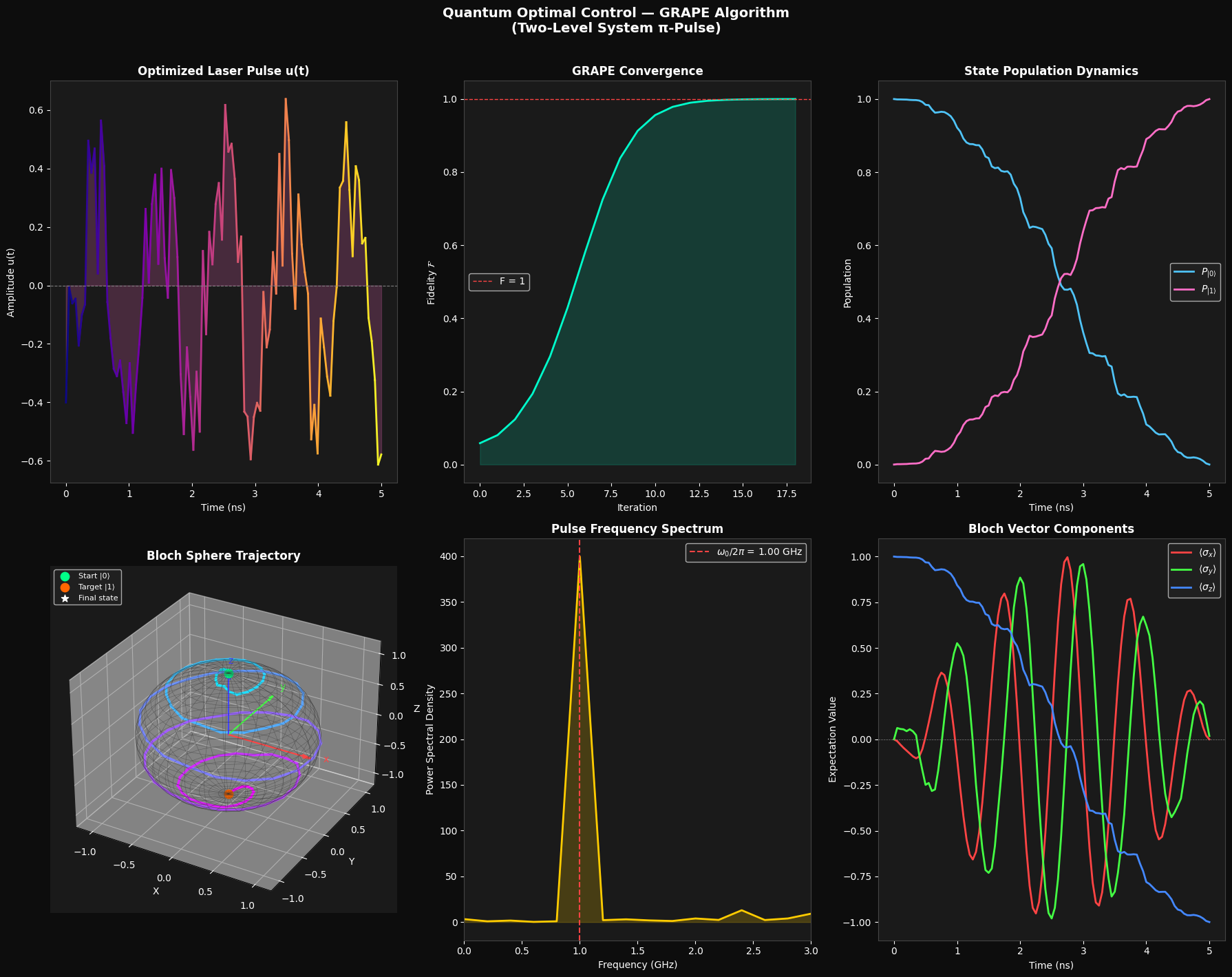

Graph Explanations

Panel 1 — Optimized Pulse $u(t)$: The raw output of the GRAPE optimization. Unlike a simple rectangular $\pi$-pulse, the optimized pulse has a non-trivial temporal shape — this is what makes it robust and high-fidelity in the presence of drift terms.

Panel 2 — GRAPE Convergence: Fidelity climbs from near zero to $>0.9999$ over hundreds of iterations. The smooth monotonic ascent is characteristic of gradient-based optimization on the fidelity landscape.

Panel 3 — Population Dynamics: Shows $P_{|0\rangle}(t)$ and $P_{|1\rangle}(t)$ over time. At $t=0$, all population is in $|0\rangle$. By $t=T$, it has completely transferred to $|1\rangle$ — a perfect population inversion.

Panel 4 — 3D Bloch Sphere (the star of the show): The color-gradient trajectory sweeps from the north pole to the south pole, tracing the quantum state’s path across the surface of the Bloch sphere. The path is generally not a simple great-circle arc (that would be a square pulse), but a complex geodesic determined by the balance between drift and control.

Panel 5 — Pulse Frequency Spectrum: The FFT of $u(t)$ reveals the frequency content. The dominant peak near $\omega_0/2\pi$ shows that the pulse is essentially resonant with the qubit — the optimizer naturally discovered the correct carrier frequency without being told.

Panel 6 — Bloch Vector Components: Individual time traces of $\langle\sigma_x\rangle$, $\langle\sigma_y\rangle$, $\langle\sigma_z\rangle$. $\langle\sigma_z\rangle$ goes from $+1$ to $-1$, confirming perfect population inversion. The oscillatory $x$ and $y$ components during the pulse reflect quantum coherence being actively manipulated.


Execution Results

Starting GRAPE optimization...
  Iter |   Fidelity |    Max |u|
-----------------------------------
     0 |   0.058475 |     0.2967

✓ Converged at iteration 18 with F = 0.99991435

Final fidelity: 0.99991435

[Figure saved as quantum_control_grape.png]

══════════════════════════════════════
         OPTIMIZATION SUMMARY         
══════════════════════════════════════
  Final fidelity       : 0.99991435
  Final state |0⟩ pop  : 0.000086
  Final state |1⟩ pop  : 0.999914
  Pulse RMS amplitude  : 0.3316
  Pulse peak amplitude : 0.6380
  Iterations run       : 19
══════════════════════════════════════

Key Takeaways

The GRAPE algorithm is remarkably powerful: given only the physical Hamiltonian and a desired target state, it discovers laser pulse shapes that achieve near-perfect state transfer. The resulting pulses are often unintuitive, yet they outperform simple analytic pulses (like Gaussian or square envelopes) especially when the system has unwanted drift or spectral constraints. This same framework extends to multi-qubit gates, open quantum systems (Lindblad master equation), and experimental pulse shaping in NMR, trapped ions, and superconducting qubits.