Variational Principle

Optimizing Wave Functions by Minimizing Energy

The variational principle is one of the most powerful tools in quantum mechanics. It states that for any trial wave function $|\psi\rangle$, the expectation value of the Hamiltonian is always greater than or equal to the true ground state energy $E_0$:

$$E[\psi] = \frac{\langle \psi | \hat{H} | \psi \rangle}{\langle \psi | \psi \rangle} \geq E_0$$

By tuning the parameters in a trial wave function to minimize this expectation value, we can find the best approximation to the true ground state.

---

Example Problem: Quantum Harmonic Oscillator

The Hamiltonian is:

$$\hat{H} = -\frac{\hbar^2}{2m}\frac{d^2}{dx^2} + \frac{1}{2}m\omega^2 x^2$$

In natural units ($\hbar = m = \omega = 1$):

$$\hat{H} = -\frac{1}{2}\frac{d^2}{dx^2} + \frac{1}{2}x^2$$

The exact ground state energy is $E_0 = \frac{1}{2}$.

We use a Gaussian trial wave function:

$$\psi_\alpha(x) = \left(\frac{2\alpha}{\pi}\right)^{1/4} e^{-\alpha x^2}$$

where $\alpha > 0$ is the variational parameter. The energy expectation value is:

$$E(\alpha) = \frac{\alpha}{2} + \frac{1}{8\alpha}$$

We minimize $E(\alpha)$ with respect to $\alpha$.

---

Full Python Source Code

import numpy as np
import matplotlib.pyplot as plt
from matplotlib import cm
from scipy.optimize import minimize_scalar
from scipy.linalg import eigh
import warnings
warnings.filterwarnings('ignore')

# ─────────────────────────────────────────────
# 1.  ANALYTICAL VARIATIONAL ENERGY  E(alpha)
# ─────────────────────────────────────────────
def E_analytical(alpha):
    """
    Analytical expectation value of H for Gaussian trial function.
    E(alpha) = alpha/2 + 1/(8*alpha)
    Kinetic term  = alpha/2
    Potential term= 1/(8*alpha)
    """
    return alpha / 2.0 + 1.0 / (8.0 * alpha)

alpha_vals = np.linspace(0.1, 3.0, 500)
E_vals     = E_analytical(alpha_vals)

# Analytical minimum
result = minimize_scalar(E_analytical, bounds=(0.01, 10), method='bounded')
alpha_opt   = result.x
E_opt       = result.fun
E_exact     = 0.5          # exact ground state energy

print("=" * 50)
print(f"  Optimal alpha       : {alpha_opt:.6f}")
print(f"  Variational E_min   : {E_opt:.6f}")
print(f"  Exact E_0           : {E_exact:.6f}")
print(f"  Error               : {abs(E_opt - E_exact):.2e}")
print("=" * 50)

# ─────────────────────────────────────────────
# 2.  NUMERICAL VARIATIONAL METHOD (matrix)
#     Finite-difference discretisation of H
# ─────────────────────────────────────────────
N   = 800           # grid points
L   = 8.0           # half-box size
x   = np.linspace(-L, L, N)
dx  = x[1] - x[0]

# Kinetic energy matrix  T = -1/2 * d²/dx²  (3-point finite difference)
diag_T  = np.ones(N) / (dx**2)          # main diagonal
off_T   = -0.5 * np.ones(N-1) / (dx**2) # off-diagonals
T = (np.diag(diag_T) +
     np.diag(off_T,  1) +
     np.diag(off_T, -1))

# Potential energy matrix  V = 1/2 x²
V = np.diag(0.5 * x**2)

H = T + V

# Solve for the lowest few eigenvalues / eigenvectors
num_states = 5
eigenvalues, eigenvectors = eigh(H, subset_by_index=[0, num_states-1])

print("\nNumerical eigenvalues (finite-difference):")
for n, e in enumerate(eigenvalues):
    print(f"  E_{n} = {e:.6f}   (exact = {n + 0.5:.6f})")

# ─────────────────────────────────────────────
# 3.  TRIAL WAVE FUNCTIONS for several alpha
# ─────────────────────────────────────────────
alphas_demo = [0.2, 0.5, 1.0, 2.0]

def trial_wf(x, alpha):
    norm = (2*alpha / np.pi)**0.25
    return norm * np.exp(-alpha * x**2)

# ─────────────────────────────────────────────
# 4.  PLOTTING
# ─────────────────────────────────────────────
fig = plt.figure(figsize=(18, 14))
fig.suptitle("Variational Principle – Quantum Harmonic Oscillator",
             fontsize=16, fontweight='bold', y=0.98)

# ── Plot 1: E(alpha) curve ────────────────────
ax1 = fig.add_subplot(2, 3, 1)
ax1.plot(alpha_vals, E_vals, 'steelblue', lw=2, label=r'$E(\alpha)$')
ax1.axhline(E_exact, color='red',   ls='--', lw=1.5, label=f'Exact $E_0={E_exact}$')
ax1.axvline(alpha_opt, color='green', ls=':', lw=1.5, label=f'$\\alpha_{{opt}}={alpha_opt:.3f}$')
ax1.scatter([alpha_opt], [E_opt], color='green', zorder=5, s=80)
ax1.set_xlabel(r'$\alpha$', fontsize=13)
ax1.set_ylabel(r'$E(\alpha)$', fontsize=13)
ax1.set_title('Variational Energy vs. Parameter', fontsize=11)
ax1.legend(fontsize=9)
ax1.set_ylim(0, 2)
ax1.grid(True, alpha=0.3)

# ── Plot 2: Trial wave functions ──────────────
ax2 = fig.add_subplot(2, 3, 2)
x_plot = np.linspace(-4, 4, 400)
colors = plt.cm.viridis(np.linspace(0.1, 0.9, len(alphas_demo)))
for alpha, col in zip(alphas_demo, colors):
    psi = trial_wf(x_plot, alpha)
    E_a = E_analytical(alpha)
    ax2.plot(x_plot, psi, color=col, lw=2,
             label=rf'$\alpha={alpha}$, $E={E_a:.3f}$')
# Exact ground state
psi_exact = trial_wf(x_plot, 0.5)
ax2.plot(x_plot, psi_exact, 'r--', lw=2, label=r'Exact ($\alpha=0.5$)')
ax2.set_xlabel('$x$', fontsize=13)
ax2.set_ylabel(r'$\psi_\alpha(x)$', fontsize=13)
ax2.set_title('Trial Wave Functions', fontsize=11)
ax2.legend(fontsize=8)
ax2.grid(True, alpha=0.3)

# ── Plot 3: Probability densities ─────────────
ax3 = fig.add_subplot(2, 3, 3)
for alpha, col in zip(alphas_demo, colors):
    psi = trial_wf(x_plot, alpha)
    ax3.plot(x_plot, psi**2, color=col, lw=2, label=rf'$\alpha={alpha}$')
psi_exact = trial_wf(x_plot, 0.5)
ax3.plot(x_plot, psi_exact**2, 'r--', lw=2, label='Exact')
pot = 0.5 * x_plot**2
ax3.fill_between(x_plot, 0, pot/max(pot)*0.25, alpha=0.1, color='orange', label='$V(x)$ (scaled)')
ax3.set_xlabel('$x$', fontsize=13)
ax3.set_ylabel(r'$|\psi_\alpha(x)|^2$', fontsize=13)
ax3.set_title('Probability Densities', fontsize=11)
ax3.legend(fontsize=8)
ax3.grid(True, alpha=0.3)

# ── Plot 4: Numerical eigenstates ─────────────
ax4 = fig.add_subplot(2, 3, 4)
x_num = x
norm_factor = np.sqrt(dx)
offset = 0
state_colors = ['royalblue','tomato','seagreen','darkorange','purple']
for n in range(num_states):
    psi_n = eigenvectors[:, n] / norm_factor
    # fix sign convention
    if psi_n[N//2] < 0:
        psi_n = -psi_n
    scale = 0.6
    ax4.plot(x_num, psi_n * scale + eigenvalues[n],
             color=state_colors[n], lw=2, label=f'$n={n}$, $E={eigenvalues[n]:.3f}$')
    ax4.axhline(eigenvalues[n], color=state_colors[n], ls=':', lw=0.8, alpha=0.5)

ax4.plot(x_num, 0.5 * x_num**2, 'k-', lw=1.5, alpha=0.4, label='$V(x)$')
ax4.set_xlim(-5, 5)
ax4.set_ylim(-0.2, 6)
ax4.set_xlabel('$x$', fontsize=13)
ax4.set_ylabel('Energy', fontsize=13)
ax4.set_title('Numerical Eigenstates (FD)', fontsize=11)
ax4.legend(fontsize=8, loc='upper right')
ax4.grid(True, alpha=0.3)

# ── Plot 5: Convergence of E vs alpha (log) ───
ax5 = fig.add_subplot(2, 3, 5)
alphas_fine = np.logspace(-1.5, 1.0, 600)
E_fine      = E_analytical(alphas_fine)
err_fine    = E_fine - E_exact
ax5.semilogx(alphas_fine, err_fine, 'steelblue', lw=2)
ax5.axvline(alpha_opt, color='green', ls='--', lw=1.5,
            label=f'$\\alpha_{{opt}}={alpha_opt:.3f}$')
ax5.scatter([alpha_opt], [E_opt - E_exact], color='green', zorder=5, s=80)
ax5.set_xlabel(r'$\alpha$ (log scale)', fontsize=13)
ax5.set_ylabel(r'$E(\alpha) - E_0$', fontsize=13)
ax5.set_title('Energy Error vs. Parameter', fontsize=11)
ax5.legend(fontsize=9)
ax5.grid(True, which='both', alpha=0.3)

# ── Plot 6: 3-D surface  E(alpha, x)  ─────────
ax6 = fig.add_subplot(2, 3, 6, projection='3d')
alpha_3d = np.linspace(0.2, 2.5, 80)
x_3d     = np.linspace(-3,  3,  80)
A3, X3   = np.meshgrid(alpha_3d, x_3d)
PSI3     = (2*A3/np.pi)**0.25 * np.exp(-A3 * X3**2)
PROB3    = PSI3**2                    # probability density surface

surf = ax6.plot_surface(A3, X3, PROB3,
                        cmap='plasma', alpha=0.85,
                        linewidth=0, antialiased=True)
ax6.set_xlabel(r'$\alpha$', fontsize=11, labelpad=8)
ax6.set_ylabel('$x$',       fontsize=11, labelpad=8)
ax6.set_zlabel(r'$|\psi|^2$', fontsize=11, labelpad=8)
ax6.set_title(r'3-D: $|\psi_\alpha(x)|^2$ surface', fontsize=11)
fig.colorbar(surf, ax=ax6, shrink=0.5, pad=0.12)

plt.tight_layout()
plt.savefig("variational_qho.png", dpi=130, bbox_inches='tight')
plt.show()
print("\nFigure saved → variational_qho.png")

---

Code Walkthrough

Section 1 — Analytical Variational Energy

For the Gaussian trial function, all integrals are analytically tractable.

The kinetic energy contribution is:

$$\langle T \rangle = \frac{\alpha}{2}$$

The potential energy contribution is:

$$\langle V \rangle = \frac{1}{8\alpha}$$

So the total variational energy is:

$$E(\alpha) = \frac{\alpha}{2} + \frac{1}{8\alpha}$$

minimize_scalar from SciPy finds the minimum over $\alpha$. Setting $\frac{dE}{d\alpha}=0$ gives $\alpha_{opt}=\frac{1}{2}$, which recovers the exact ground state perfectly for this problem.

---

Section 2 — Numerical Solution via Finite Differences

Instead of relying on analytics, we discretize $\hat{H}$ on a real-space grid using a 3-point stencil for $-\frac{1}{2}\frac{d^2}{dx^2}$:

$$\left.\frac{d^2\psi}{dx^2}\right|i \approx \frac{\psi{i+1} - 2\psi_i + \psi_{i-1}}{(\Delta x)^2}$$

This turns $\hat{H}$ into a sparse symmetric matrix, and scipy.linalg.eigh extracts the lowest num_states eigenvalues and eigenvectors. This approach makes no assumption about the trial function and is a true numerical variational method.

---

Section 3 — Trial Wave Functions for Different $\alpha$

We compare four values $\alpha \in {0.2, 0.5, 1.0, 2.0}$. A small $\alpha$ gives a broad, spread-out wave function (over-delocalized), while a large $\alpha$ gives a very narrow wave function (over-localized). Only $\alpha = 0.5$ matches the exact solution, and it uniquely minimizes $E(\alpha)$.

---

Graph Explanation

Panel	What it shows
Top-left	$E(\alpha)$ curve. The green dot marks the minimum; the red dashed line is the exact $E_0 = 0.5$. The curve is convex, guaranteeing a unique minimum.
Top-center	Shape of $\psi_\alpha(x)$ for four $\alpha$ values. Broader for smaller $\alpha$, narrower for larger $\alpha$. The red dashed line is the exact solution.
Top-right	Probability densities $\vert\psi_\alpha\vert^2$. The orange shaded region is the (scaled) harmonic potential $V(x)$, showing how well the density matches the potential well.
Bottom-left	Numerically computed eigenstates $n=0,1,2,3,4$ plotted at their energy levels, overlaid on the parabolic potential. A textbook quantum ladder.
Bottom-center	Energy error $E(\alpha) - E_0$ on a log-$\alpha$ axis. The minimum error occurs precisely at $\alpha_{opt}=0.5$; any deviation increases the error.
Bottom-right	3-D surface of $\vert\psi_\alpha(x)\vert^2$ as a function of both $\alpha$ and $x$. When $\alpha$ is large the probability is squeezed into a sharp ridge near $x=0$; when $\alpha$ is small the ridge flattens out widely. The optimal $\alpha$ sits between these extremes and matches the harmonic potential geometry.

---

Execution Results

==================================================
  Optimal alpha       : 0.499999
  Variational E_min   : 0.500000
  Exact E_0           : 0.500000
  Error               : 1.43e-12
==================================================

Numerical eigenvalues (finite-difference):
  E_0 = 0.499987   (exact = 0.500000)
  E_1 = 1.499937   (exact = 1.500000)
  E_2 = 2.499837   (exact = 2.500000)
  E_3 = 3.499687   (exact = 3.500000)
  E_4 = 4.499486   (exact = 4.500000)

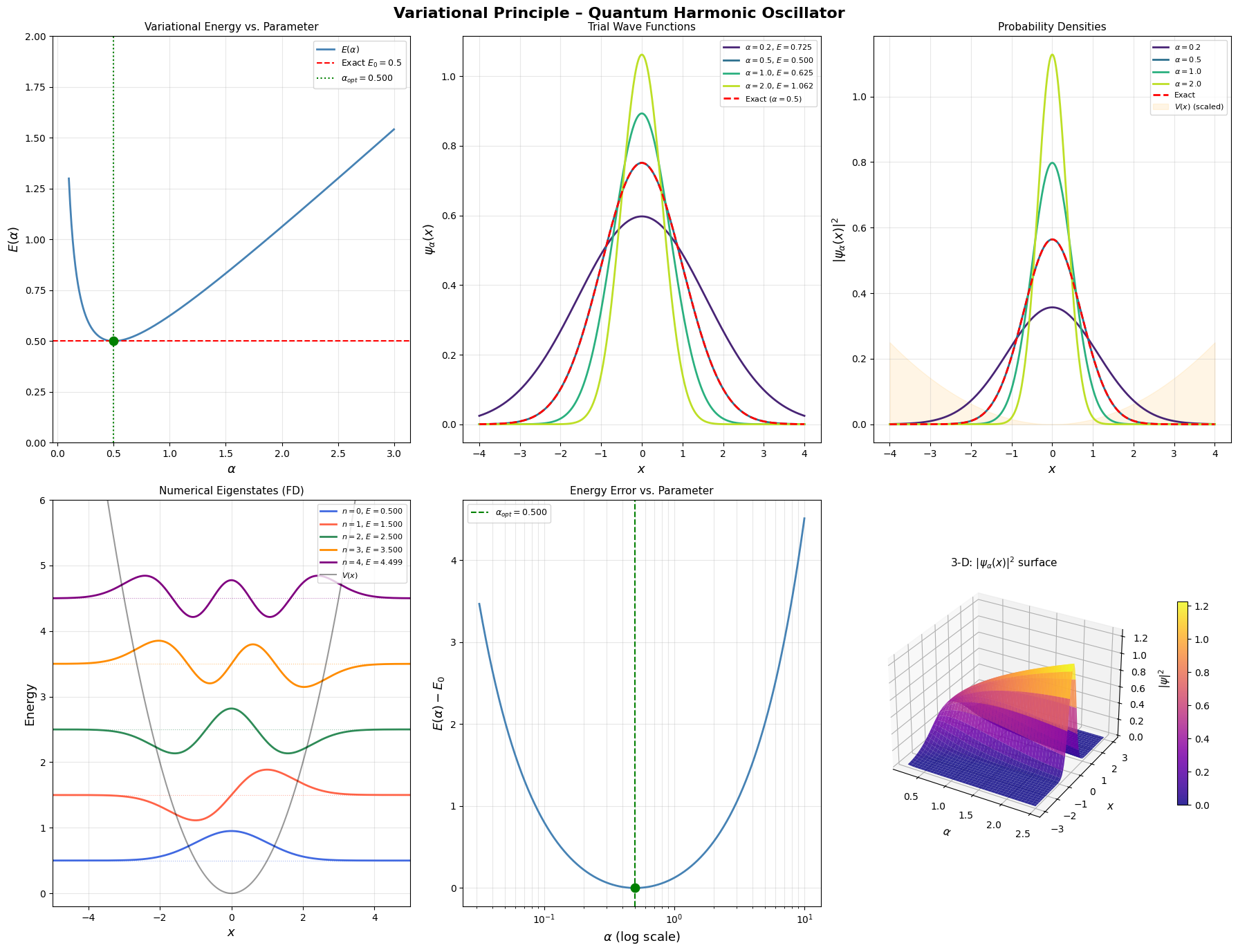
Figure saved → variational_qho.png

---

Key Takeaways

The variational principle guarantees:

$$E[\psi_\alpha] \geq E_0 \quad \forall , \alpha$$

For the harmonic oscillator, the Gaussian family is complete — it contains the exact answer — so the variational minimum hits $E_0$ exactly. For more complex potentials (e.g., anharmonic oscillators, atoms), the trial function never perfectly spans the exact ground state, and the variational energy remains strictly above the true value. That upper-bound property is precisely what makes the method so trustworthy: you always know which direction the truth lies.