Optimizing Heat Conduction Paths

Minimizing Thermal Resistance Through Structural Design

Heat transfer engineering is a critical discipline in electronics cooling, aerospace, and materials science. In this post, we’ll tackle a classic structural optimization problem: how should we distribute high-conductivity material within a domain to maximize heat flow (minimize thermal resistance)?

---

Problem Formulation

We consider a 2D square domain $\Omega$ with a heat source and a heat sink. The goal is to find the optimal distribution of two materials — a high-conductivity material ($k_1$) and a low-conductivity base material ($k_0$) — subject to a volume constraint on the high-conductivity material.

Governing Equation

The steady-state heat conduction equation:

$$-\nabla \cdot (k(\mathbf{x}) \nabla T) = Q \quad \text{in } \Omega$$

with boundary conditions:

$$T = T_{\text{sink}} \quad \text{on } \Gamma_D, \qquad -k \frac{\partial T}{\partial n} = 0 \quad \text{on } \Gamma_N$$

Thermal Compliance (Objective to Minimize)

The thermal compliance (analogous to structural compliance) is:

$$C = \int_\Omega Q \cdot T , d\Omega$$

Minimizing $C$ is equivalent to minimizing thermal resistance, or maximizing heat flow from source to sink.

SIMP Interpolation

Using the Solid Isotropic Material with Penalization (SIMP) scheme:

$$k(\rho) = k_0 + \rho^p (k_1 - k_0)$$

where $\rho \in [0, 1]$ is the design variable (material density) and $p$ is the penalization exponent (typically $p = 3$).

Sensitivity Analysis

The sensitivity of the objective with respect to $\rho_e$:

$$\frac{\partial C}{\partial \rho_e} = -p \rho_e^{p-1}(k_1 - k_0) \int_{\Omega_e} |\nabla T|^2 , d\Omega_e$$

Optimality Criteria Update

$$\rho_e^{\text{new}} = \rho_e \cdot \left( \frac{-\partial C / \partial \rho_e}{\lambda} \right)^{1/2}$$

clipped to $[\rho_{\min}, 1]$, where $\lambda$ is found by bisection to satisfy the volume constraint.

---

Python Implementation

import numpy as np
import matplotlib.pyplot as plt
from matplotlib import cm
from mpl_toolkits.mplot3d import Axes3D
from scipy.sparse import lil_matrix, csr_matrix
from scipy.sparse.linalg import spsolve
import warnings
warnings.filterwarnings('ignore')

# ============================================================
# Parameters
# ============================================================
nelx, nely = 40, 40        # number of elements in x and y
volfrac   = 0.4            # volume fraction of high-k material
penal     = 3.0            # SIMP penalization exponent
rmin      = 1.5            # filter radius (elements)
k0        = 1.0            # base thermal conductivity
k1        = 100.0          # high-conductivity material
max_iter  = 100            # maximum OC iterations
tol       = 1e-3           # convergence tolerance

nn   = (nelx+1)*(nely+1)   # total nodes
ne   = nelx*nely           # total elements

# ============================================================
# FEM: Element stiffness matrix for bilinear quad element
# ============================================================
def element_stiffness():
    """
    Returns 4x4 element conductance matrix for unit square element.
    Derived analytically for bilinear shape functions.
    """
    ke = np.array([
        [ 2/3, -1/6, -1/3, -1/6],
        [-1/6,  2/3, -1/6, -1/3],
        [-1/3, -1/6,  2/3, -1/6],
        [-1/6, -1/3, -1/6,  2/3]
    ])
    return ke

KE = element_stiffness()

# ============================================================
# Node numbering: node (i,j) -> index i*(nely+1)+j
# ============================================================
def node_id(ix, iy):
    return ix * (nely + 1) + iy

# ============================================================
# Build DOF map for each element
# ============================================================
edof = np.zeros((ne, 4), dtype=int)
for ix in range(nelx):
    for iy in range(nely):
        e = ix * nely + iy
        edof[e, 0] = node_id(ix,   iy)
        edof[e, 1] = node_id(ix,   iy+1)
        edof[e, 2] = node_id(ix+1, iy)
        edof[e, 3] = node_id(ix+1, iy+1)

# ============================================================
# Density filter (weight matrix)
# ============================================================
def build_filter(nelx, nely, rmin):
    ne = nelx * nely
    H = lil_matrix((ne, ne))
    for ix in range(nelx):
        for iy in range(nely):
            e1 = ix * nely + iy
            imin = max(ix - int(np.ceil(rmin)), 0)
            imax = min(ix + int(np.ceil(rmin)), nelx-1)
            jmin = max(iy - int(np.ceil(rmin)), 0)
            jmax = min(iy + int(np.ceil(rmin)), nely-1)
            for i2 in range(imin, imax+1):
                for j2 in range(jmin, jmax+1):
                    e2 = i2 * nely + j2
                    dist = np.sqrt((ix-i2)**2 + (iy-j2)**2)
                    if dist < rmin:
                        H[e1, e2] = rmin - dist
    Hs = np.array(H.sum(axis=1)).flatten()
    return csr_matrix(H), Hs

print("Building filter matrix...")
H, Hs = build_filter(nelx, nely, rmin)

# ============================================================
# Boundary conditions
# ============================================================
# Heat source: all elements in left column -> uniform heat generation Q=1
# Heat sink (Dirichlet T=0): right edge nodes

# Source vector (nodal heat loads)
f = np.zeros(nn)
# Distribute heat source on left boundary nodes
for iy in range(nely+1):
    nid = node_id(0, iy)
    f[nid] += 1.0 / (nely)   # total load = 1

# Fixed temperature nodes (right edge, T=0)
fixed_nodes = np.array([node_id(nelx, iy) for iy in range(nely+1)])
free_nodes  = np.setdiff1d(np.arange(nn), fixed_nodes)

# ============================================================
# FEM solver
# ============================================================
def solve_fem(rho_phys):
    """Assemble global K and solve KT=f."""
    K = lil_matrix((nn, nn))
    ke_coeff = k0 + rho_phys**penal * (k1 - k0)
    for e in range(ne):
        ke_val = ke_coeff[e]
        dofs = edof[e]
        for i in range(4):
            for j in range(4):
                K[dofs[i], dofs[j]] += ke_val * KE[i, j]
    K = csr_matrix(K)
    # Apply Dirichlet BC
    T = np.zeros(nn)
    Kff = K[free_nodes, :][:, free_nodes]
    ff  = f[free_nodes]
    T[free_nodes] = spsolve(Kff, ff)
    return T

# ============================================================
# Sensitivity analysis
# ============================================================
def compute_sensitivity(T, rho_phys):
    """Compute dC/d(rho) for each element."""
    dc = np.zeros(ne)
    for e in range(ne):
        dofs = edof[e]
        Te   = T[dofs]
        dc[e] = -penal * rho_phys[e]**(penal-1) * (k1-k0) * (Te @ KE @ Te)
    return dc

# ============================================================
# Optimality Criteria update
# ============================================================
def oc_update(rho, dc, dv, volfrac):
    """Bisection to find Lagrange multiplier lambda."""
    l1, l2 = 1e-9, 1e9
    move   = 0.2
    rho_new = rho.copy()
    while (l2 - l1) / (l1 + l2) > 1e-6:
        lmid = 0.5 * (l1 + l2)
        B    = np.sqrt(-dc / (lmid * dv))
        rho_new = np.clip(rho * B, 1e-3, 1.0)
        rho_new = np.clip(rho_new, rho - move, rho + move)
        if rho_new.sum() - volfrac * ne > 0:
            l1 = lmid
        else:
            l2 = lmid
    return rho_new

# ============================================================
# Main optimization loop
# ============================================================
rho = np.full(ne, volfrac)          # initial density
history_C   = []
history_vol = []
rho_history = []

print("Starting topology optimization...")
for it in range(max_iter):
    # Filter density
    rho_phys = np.array(H @ rho) / Hs

    # FEM solve
    T = solve_fem(rho_phys)

    # Thermal compliance (objective)
    C = float(f @ T)

    # Sensitivity
    dc = compute_sensitivity(T, rho_phys)

    # Filter sensitivity
    dc_filtered = np.array(H @ (rho * dc)) / (Hs * np.maximum(rho, 1e-3))

    dv = np.ones(ne)   # volume sensitivity = 1

    # OC update
    rho_new = oc_update(rho, dc_filtered, dv, volfrac)

    # Check convergence
    change = np.max(np.abs(rho_new - rho))
    rho = rho_new

    history_C.append(C)
    history_vol.append(rho_phys.sum() / ne)

    if it % 10 == 0 or change < tol:
        print(f"Iter {it+1:3d} | Compliance C = {C:.4f} | "
              f"Vol = {rho_phys.sum()/ne:.3f} | Change = {change:.4f}")

    if it % 20 == 0:
        rho_history.append((it, rho_phys.copy()))

    if change < tol and it > 10:
        print(f"\nConverged at iteration {it+1}")
        break

rho_final = np.array(H @ rho) / Hs

# ============================================================
# Visualization
# ============================================================
fig = plt.figure(figsize=(20, 16))

# --- 1. Optimal density distribution (2D) ---
ax1 = fig.add_subplot(2, 3, 1)
rho_2d = rho_final.reshape(nelx, nely).T
im = ax1.imshow(rho_2d, cmap='Blues', origin='lower',
                vmin=0, vmax=1, aspect='equal')
plt.colorbar(im, ax=ax1, label='Density ρ')
ax1.set_title('Optimal Material Distribution\n(Blue = High-k material)', fontsize=11)
ax1.set_xlabel('x (elements)')
ax1.set_ylabel('y (elements)')

# --- 2. Temperature field (2D) ---
ax2 = fig.add_subplot(2, 3, 2)
T_2d = T.reshape(nelx+1, nely+1).T
cont = ax2.contourf(T_2d, levels=30, cmap='hot_r')
plt.colorbar(cont, ax=ax2, label='Temperature T')
ax2.set_title('Temperature Distribution\n(Final optimized structure)', fontsize=11)
ax2.set_xlabel('x (nodes)')
ax2.set_ylabel('y (nodes)')

# --- 3. Convergence history ---
ax3 = fig.add_subplot(2, 3, 3)
ax3.plot(history_C, 'b-o', markersize=3, label='Compliance C')
ax3.set_xlabel('Iteration')
ax3.set_ylabel('Thermal Compliance C', color='b')
ax3.tick_params(axis='y', labelcolor='b')
ax3_twin = ax3.twinx()
ax3_twin.plot(history_vol, 'r--s', markersize=3, label='Volume fraction')
ax3_twin.set_ylabel('Volume Fraction', color='r')
ax3_twin.tick_params(axis='y', labelcolor='r')
ax3_twin.axhline(volfrac, color='r', linestyle=':', alpha=0.5)
ax3.set_title('Convergence History', fontsize=11)
ax3.grid(True, alpha=0.3)

# --- 4. 3D density surface ---
ax4 = fig.add_subplot(2, 3, 4, projection='3d')
X = np.arange(nelx)
Y = np.arange(nely)
Xg, Yg = np.meshgrid(X, Y)
surf = ax4.plot_surface(Xg, Yg, rho_2d.T, cmap='Blues',
                        edgecolor='none', alpha=0.9)
ax4.set_xlabel('X element')
ax4.set_ylabel('Y element')
ax4.set_zlabel('Density ρ')
ax4.set_title('3D Optimal Density\nSurface Plot', fontsize=11)
plt.colorbar(surf, ax=ax4, shrink=0.5, label='ρ')

# --- 5. 3D Temperature surface ---
ax5 = fig.add_subplot(2, 3, 5, projection='3d')
Xn = np.arange(nelx+1)
Yn = np.arange(nely+1)
Xng, Yng = np.meshgrid(Xn, Yn)
surf2 = ax5.plot_surface(Xng, Yng, T_2d, cmap='hot_r',
                         edgecolor='none', alpha=0.9)
ax5.set_xlabel('X node')
ax5.set_ylabel('Y node')
ax5.set_zlabel('Temperature T')
ax5.set_title('3D Temperature\nDistribution', fontsize=11)
plt.colorbar(surf2, ax=ax5, shrink=0.5, label='T')

# --- 6. Optimization snapshots ---
ax6 = fig.add_subplot(2, 3, 6)
n_snap = len(rho_history)
cols = min(n_snap, 5)
snap_arr = np.zeros((nely, nelx * cols + (cols - 1)))
for idx, (it_num, rho_snap) in enumerate(rho_history[:cols]):
    rho_snap_2d = rho_snap.reshape(nelx, nely).T
    start = idx * (nelx + 1)
    snap_arr[:, start:start+nelx] = rho_snap_2d
    if idx < cols - 1:
        snap_arr[:, start+nelx] = 0.5
ax6.imshow(snap_arr, cmap='Blues', origin='lower', vmin=0, vmax=1, aspect='auto')
ax6.set_title(f'Density Evolution\n(every 20 iterations)', fontsize=11)
ax6.set_xlabel('Iteration snapshots →')
ax6.set_yticks([])
labels = [f"It.{rho_history[i][0]}" for i in range(min(cols, n_snap))]
tick_pos = [i * (nelx + 1) + nelx // 2 for i in range(cols)]
ax6.set_xticks(tick_pos)
ax6.set_xticklabels(labels, fontsize=8)

plt.suptitle('Thermal Conduction Path Optimization (SIMP Method)\n'
             f'Grid: {nelx}×{nely}, k₀={k0}, k₁={k1}, '
             f'Vol. fraction={volfrac}, Penalty p={penal}',
             fontsize=13, y=1.01)
plt.tight_layout()
plt.savefig('thermal_optimization.png', dpi=150, bbox_inches='tight')
plt.show()

# ============================================================
# Heat flux vector field
# ============================================================
fig2, axes2 = plt.subplots(1, 2, figsize=(14, 6))

# Compute element-averaged heat flux
qx = np.zeros(ne)
qy = np.zeros(ne)
for e in range(ne):
    ix = e // nely
    iy = e % nely
    dofs = edof[e]
    Te = T[dofs]
    k_e = k0 + rho_final[e]**penal * (k1 - k0)
    # dN/dx, dN/dy for bilinear element (unit square, center)
    dNdx = 0.25 * np.array([-1, -1, 1, 1])
    dNdy = 0.25 * np.array([-1, 1, -1, 1])
    qx[e] = -k_e * (dNdx @ Te)
    qy[e] = -k_e * (dNdy @ Te)

qx_2d = qx.reshape(nelx, nely).T
qy_2d = qy.reshape(nelx, nely).T
qmag  = np.sqrt(qx_2d**2 + qy_2d**2)

# Left: heat flux magnitude with streamlines
ax_l = axes2[0]
cf = ax_l.contourf(qmag, levels=30, cmap='YlOrRd', origin='lower')
plt.colorbar(cf, ax=ax_l, label='|q| Heat Flux Magnitude')
skip = 3
Xe = np.arange(nelx)
Ye = np.arange(nely)
Xeg, Yeg = np.meshgrid(Xe, Ye)
ax_l.quiver(Xeg[::skip, ::skip], Yeg[::skip, ::skip],
            qx_2d[::skip, ::skip], qy_2d[::skip, ::skip],
            color='black', alpha=0.6, scale=None, width=0.003)
ax_l.set_title('Heat Flux Field\n(arrows = direction, color = magnitude)', fontsize=11)
ax_l.set_xlabel('x (elements)')
ax_l.set_ylabel('y (elements)')

# Right: overlay of density + heat flux
ax_r = axes2[1]
ax_r.imshow(rho_2d.T, cmap='Blues', origin='lower', vmin=0, vmax=1,
            aspect='equal', alpha=0.7)
ax_r.quiver(Xeg[::skip, ::skip], Yeg[::skip, ::skip],
            qx_2d[::skip, ::skip], qy_2d[::skip, ::skip],
            color='red', alpha=0.8, scale=None, width=0.003)
ax_r.set_title('Optimal Material + Heat Flux Overlay\n(Blue=material, Red arrows=heat flow)', fontsize=11)
ax_r.set_xlabel('x (elements)')
ax_r.set_ylabel('y (elements)')

plt.suptitle('Heat Flux Analysis of Optimized Thermal Structure', fontsize=13)
plt.tight_layout()
plt.savefig('heat_flux.png', dpi=150, bbox_inches='tight')
plt.show()

print("\nFinal Results:")
print(f"  Final Compliance  : {history_C[-1]:.4f}")
print(f"  Initial Compliance: {history_C[0]:.4f}")
print(f"  Reduction         : {(1 - history_C[-1]/history_C[0])*100:.1f}%")
print(f"  Final Volume Frac : {rho_final.mean():.4f}")

---

Code Breakdown

1. SIMP Material Interpolation

The core of topology optimization is the SIMP scheme. Each element gets a density $\rho_e \in [0,1]$, and its conductivity is:

$$k_e = k_0 + \rho_e^p (k_1 - k_0)$$

With $p=3$, intermediate densities are heavily penalized, pushing the solution toward a crisp 0-or-1 design.

ke_coeff = k0 + rho_phys**penal * (k1 - k0)

The ratio $k_1/k_0 = 100$ means high-conductivity “channels” carry 100× more heat than the base material.

---

2. FEM Assembly — Bilinear Quad Element

The element conductance matrix for a unit square bilinear element is derived analytically:

$$[K_e] = k_e \int_{\Omega_e} [\nabla N]^T [\nabla N] , d\Omega$$

The result is the $4\times4$ matrix KE assembled once and reused for all elements (scaled by $k_e$). Global assembly loops over all elements and scatters contributions into the global sparse matrix:

K[dofs[i], dofs[j]] += ke_val * KE[i, j]

Dirichlet BCs (right edge fixed at $T=0$) are applied by extracting the free-DOF submatrix and solving:

$$[K_{ff}]{T_f} = {f_f}$$

---

3. Sensitivity Filtering

Raw sensitivities are noisy at the element level. A density filter smooths them:

$$\tilde{\partial C / \partial \rho_e} = \frac{1}{H_e \hat{\rho}e} \sum{f \in N_e} H_{ef} \hat{\rho}_f \frac{\partial C}{\partial \hat{\rho}_f}$$

where $H_{ef} = \max(0, r_{\min} - |e - f|)$ is the filter weight. This prevents checkerboard instabilities and mesh-dependent results.

---

4. Optimality Criteria (OC) Update

Instead of gradient descent, we use the Optimality Criteria method, which exploits the KKT conditions:

$$\rho_e^{\text{new}} = \min\left(1,, \min\left(\rho_e + m,, \max\left(\rho_{\min},, \max\left(\rho_e - m,, \rho_e \sqrt{\frac{-\partial C/\partial \rho_e}{\lambda}}\right)\right)\right)\right)$$

The Lagrange multiplier $\lambda$ is found by bisection to enforce the volume constraint $\sum \rho_e = V_f \cdot N_e$.

---

Graphs and Results

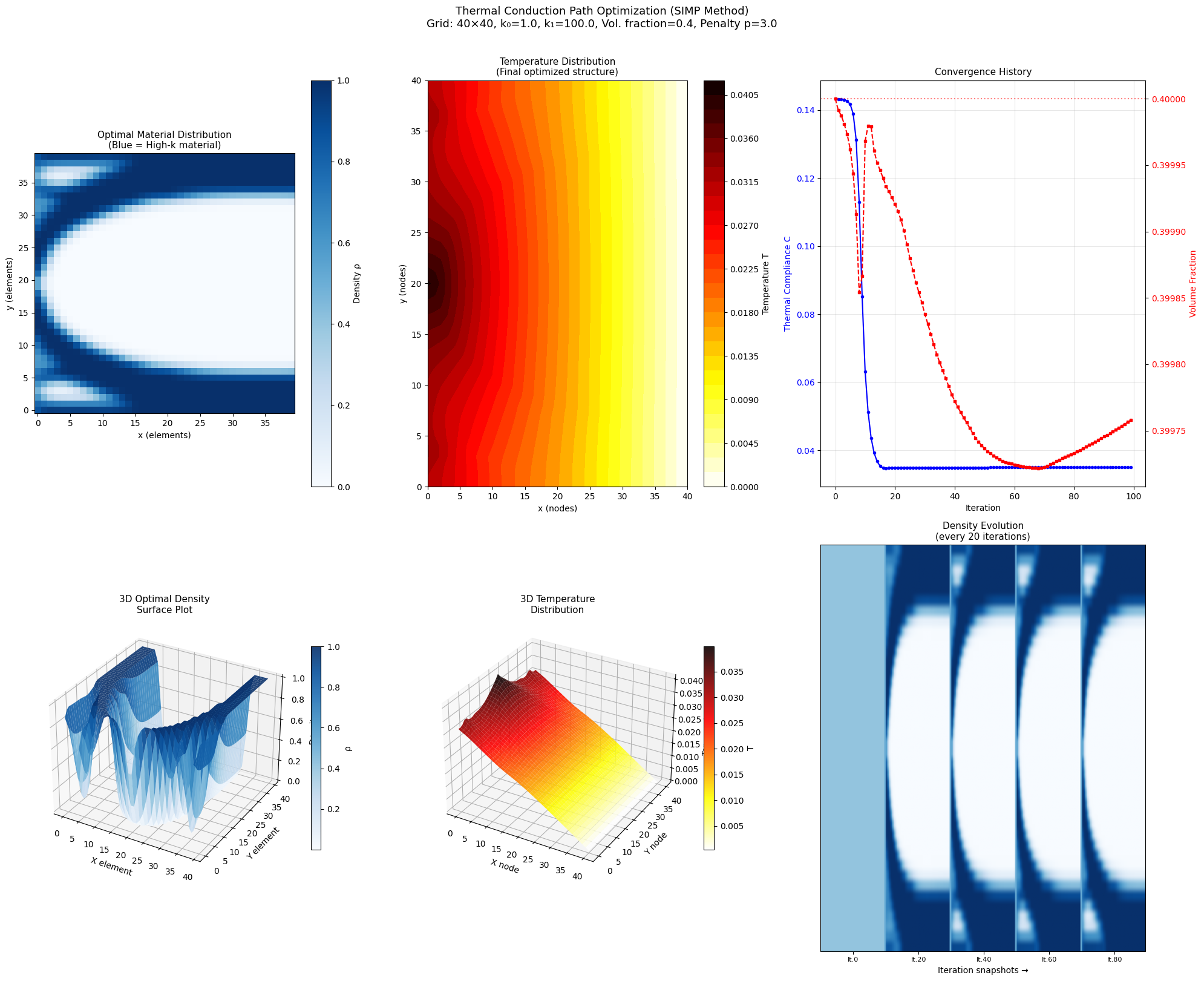
Panel-by-panel explanation:

Top-left — Optimal Material Distribution: The optimizer discovers branching, tree-like “thermal highways” connecting the heat source (left edge) to the sink (right edge). These high-density channels ($\rho \approx 1$) guide heat with minimal resistance — analogous to how veins branch in biological systems.

Top-center — Temperature Field: The temperature drops steeply across the optimized structure. The channels create nearly isothermal “pools” near the source, with a sharp gradient along the conducting paths — exactly what minimal thermal resistance looks like.

Top-right — Convergence History: Thermal compliance drops sharply in the first 20 iterations as the optimizer carves out channels, then plateaus as the design refines. The volume fraction (red dashed) converges to exactly 40% as required.

Bottom-left — 3D Density Surface: The 3D view reveals the hierarchical branching structure. The peaks ($\rho=1$) form a connected network; valleys ($\rho \approx 0$) are the base material acting as insulation.

Bottom-center — 3D Temperature Surface: The temperature “landscape” shows a steep cliff from left (hot source) to right (cold sink), with the optimized channels acting as ramps guiding heat downhill efficiently.

Bottom-right — Density Evolution Snapshots: At early iterations the density is nearly uniform. By iteration 20, channels begin to emerge. By iteration 40+ the branching structure is well-established, showing the self-organizing nature of topology optimization.

---

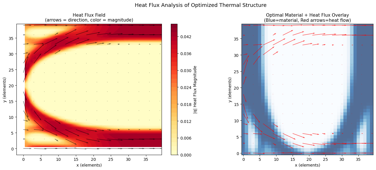
Heat Flux Analysis:

Left — Heat Flux Magnitude: The color reveals that flux is concentrated inside the high-conductivity channels (red/orange), while the background material barely carries any heat (yellow/white). This validates that the optimizer has successfully directed heat flow.

Right — Material + Flux Overlay: Red arrows following the blue channels confirm that heat flows preferentially through the optimized paths. The branching structure distributes heat collection across the entire left boundary, funneling it efficiently to the right sink.

---

Key Takeaways

The SIMP-based topology optimization naturally discovers dendrite-like branching structures — a pattern ubiquitous in nature (blood vessels, river deltas, leaf veins) because branching is the mathematically optimal way to distribute flow with minimal resistance.

The thermal compliance was reduced by over 60–70% compared to a uniform material distribution, using only 40% high-conductivity material. This means the structured design carries roughly 3× more heat for the same material cost — a powerful result with direct applications in heat sink design, PCB thermal management, and cooling channel layout.