Maximizing Heat Engine Efficiency

Theory, Examples & Python Visualization

What Is a Heat Engine?

A heat engine converts thermal energy into mechanical work by operating between a hot reservoir at temperature $T_H$ and a cold reservoir at temperature $T_C$. The maximum theoretical efficiency is the Carnot efficiency:

$$\eta_{Carnot} = 1 - \frac{T_C}{T_H}$$

But Carnot efficiency is achieved only at zero power output (quasi-static process). In real engines, we want to maximize power output, not just efficiency. This leads to the Curzon-Ahlborn efficiency:

$$\eta_{CA} = 1 - \sqrt{\frac{T_C}{T_H}}$$


The Problem Setup

Consider a heat engine with:

  • Hot reservoir: $T_H$ (variable, 400 K–1200 K)
  • Cold reservoir: $T_C = 300$ K (fixed, ambient)
  • Internal irreversibilities modeled by a heat conductance parameter $K$

The power output of an endoreversible engine is:

$$P = K \cdot \frac{(T_H - T_C)^2}{4 T_H}$$

The efficiency at maximum power is:

$$\eta_{MP} = 1 - \sqrt{\frac{T_C}{T_H}} = \eta_{CA}$$

We want to:

  1. Find $\eta_{CA}$ for various $T_H$
  2. Compare it with $\eta_{Carnot}$
  3. Visualize power as a function of efficiency
  4. Show a 3D surface of power vs. $T_H$ and $T_C$

Python Source Code

1
2
3
4
5
6
7
8
9
10
11
12
13
14
15
16
17
18
19
20
21
22
23
24
25
26
27
28
29
30
31
32
33
34
35
36
37
38
39
40
41
42
43
44
45
46
47
48
49
50
51
52
53
54
55
56
57
58
59
60
61
62
63
64
65
66
67
68
69
70
71
72
73
74
75
76
77
78
79
80
81
82
83
84
85
86
87
88
89
90
91
92
93
94
95
96
97
98
99
100
101
102
103
104
105
106
107
108
109
110
111
112
113
114
115
116
117
118
119
120
121
122
123
124
125
126
127
128
129
130
131
132
133
134
135
136
137
138
139
140
141
142
143
144
145
146
147
148
149
150
151
152
153
154
155
156
157
158
import numpy as np
import matplotlib.pyplot as plt
from mpl_toolkits.mplot3d import Axes3D
from scipy.optimize import minimize_scalar

# ============================================================
# Parameters
# ============================================================
TC_fixed = 300.0 # Cold reservoir temperature [K]
TH_array = np.linspace(400, 1200, 500) # Hot reservoir range [K]
K = 1.0 # Heat conductance [W/K] (normalized)

# ============================================================
# Functions
# ============================================================

def carnot_efficiency(TH, TC):
return 1.0 - TC / TH

def curzon_ahlborn_efficiency(TH, TC):
return 1.0 - np.sqrt(TC / TH)

def power_output(TH, TC, K=1.0):
"""Power of endoreversible engine at max-power operating point."""
return K * (TH - TC)**2 / (4.0 * TH)

def power_vs_efficiency(eta, TH, TC, K=1.0):
"""
Express power as function of efficiency eta for given TH, TC.
Derived from: eta = 1 - Q_C/Q_H, and endoreversible constraint.
P(eta) = K * TC * eta * (1 - eta/eta_Carnot) / (1 - eta)
"""
eta_C = carnot_efficiency(TH, TC)
# Avoid division by zero
with np.errstate(divide='ignore', invalid='ignore'):
P = np.where(
(eta < eta_C) & (eta >= 0),
K * TC * eta * (1.0 - eta / eta_C) / (1.0 - eta + 1e-12),
0.0
)
return P

# ============================================================
# 1. Compute efficiencies vs TH
# ============================================================
eta_carnot = carnot_efficiency(TH_array, TC_fixed)
eta_ca = curzon_ahlborn_efficiency(TH_array, TC_fixed)
P_max = power_output(TH_array, TC_fixed, K)

# ============================================================
# 2. Specific example: TH = 800 K, TC = 300 K
# ============================================================
TH_ex, TC_ex = 800.0, 300.0
eta_C_ex = carnot_efficiency(TH_ex, TC_ex)
eta_CA_ex = curzon_ahlborn_efficiency(TH_ex, TC_ex)
P_ex = power_output(TH_ex, TC_ex, K)

print("=" * 50)
print(f"Example: TH = {TH_ex} K, TC = {TC_ex} K")
print(f" Carnot efficiency : {eta_C_ex:.4f} ({eta_C_ex*100:.2f}%)")
print(f" Curzon-Ahlborn (max-P) : {eta_CA_ex:.4f} ({eta_CA_ex*100:.2f}%)")
print(f" Max power output (norm) : {P_ex:.4f} W")
print("=" * 50)

# Verify numerically via scipy
eta_vals = np.linspace(0.001, eta_C_ex - 0.001, 2000)
P_vals = power_vs_efficiency(eta_vals, TH_ex, TC_ex, K)
idx_max = np.argmax(P_vals)
print(f" Numerical max-P at eta : {eta_vals[idx_max]:.4f} ({eta_vals[idx_max]*100:.2f}%)")
print(f" Analytical CA eta : {eta_CA_ex:.4f}")

# ============================================================
# Figure 1: Efficiency vs TH (2D)
# ============================================================
fig, axes = plt.subplots(1, 2, figsize=(14, 5))
fig.suptitle("Heat Engine Efficiency Maximization", fontsize=14, fontweight='bold')

ax = axes[0]
ax.plot(TH_array, eta_carnot * 100, 'r-', lw=2, label=r'Carnot $\eta_C = 1 - T_C/T_H$')
ax.plot(TH_array, eta_ca * 100, 'b--', lw=2, label=r'Curzon-Ahlborn $\eta_{CA} = 1 - \sqrt{T_C/T_H}$')
ax.axvline(TH_ex, color='gray', ls=':', lw=1)
ax.plot(TH_ex, eta_C_ex * 100, 'ro', ms=8, label=f'Carnot @ {TH_ex}K = {eta_C_ex*100:.1f}%')
ax.plot(TH_ex, eta_CA_ex * 100, 'bs', ms=8, label=f'CA @ {TH_ex}K = {eta_CA_ex*100:.1f}%')
ax.set_xlabel(r'$T_H$ [K]', fontsize=12)
ax.set_ylabel('Efficiency [%]', fontsize=12)
ax.set_title(r'Efficiency vs $T_H$ ($T_C = 300$ K)', fontsize=12)
ax.legend(fontsize=9)
ax.grid(True, alpha=0.3)

# ============================================================
# Figure 2: Power vs Efficiency (P-eta curve)
# ============================================================
ax2 = axes[1]
for TH_i, col in zip([500, 800, 1100], ['green', 'blue', 'red']):
eta_C_i = carnot_efficiency(TH_i, TC_fixed)
eta_CA_i = curzon_ahlborn_efficiency(TH_i, TC_fixed)
e_range = np.linspace(0.001, eta_C_i - 0.001, 1000)
P_range = power_vs_efficiency(e_range, TH_i, TC_fixed, K)
P_range = P_range / (P_range.max() + 1e-12) # normalize
ax2.plot(e_range * 100, P_range, color=col, lw=2, label=f'$T_H$ = {TH_i} K')
# Mark CA point
P_CA_i = power_vs_efficiency(np.array([eta_CA_i]), TH_i, TC_fixed, K)
P_CA_norm = P_CA_i / (power_vs_efficiency(e_range, TH_i, TC_fixed, K).max() + 1e-12)
ax2.plot(eta_CA_i * 100, P_CA_norm, 'k^', ms=8)

ax2.set_xlabel('Efficiency [%]', fontsize=12)
ax2.set_ylabel('Normalized Power', fontsize=12)
ax2.set_title(r'Power vs Efficiency ($\triangle$ = CA max-power point)', fontsize=12)
ax2.legend(fontsize=10)
ax2.grid(True, alpha=0.3)

plt.tight_layout()
plt.savefig('heat_engine_2d.png', dpi=150, bbox_inches='tight')
plt.show()

# ============================================================
# Figure 3: 3D surface — Power vs TH and TC
# ============================================================
TH_3d = np.linspace(400, 1200, 150)
TC_3d = np.linspace(200, 600, 150)
TH_mg, TC_mg = np.meshgrid(TH_3d, TC_3d)

# Only physical: TH > TC
P_3d = np.where(TH_mg > TC_mg + 10,
K * (TH_mg - TC_mg)**2 / (4.0 * TH_mg),
np.nan)

fig3d = plt.figure(figsize=(13, 7))

# — Surface plot
ax3 = fig3d.add_subplot(121, projection='3d')
surf = ax3.plot_surface(TH_mg, TC_mg, P_3d, cmap='plasma', alpha=0.85, linewidth=0)
fig3d.colorbar(surf, ax=ax3, shrink=0.5, label='Max Power [W]')
ax3.set_xlabel(r'$T_H$ [K]', fontsize=10)
ax3.set_ylabel(r'$T_C$ [K]', fontsize=10)
ax3.set_zlabel('Max Power [W]', fontsize=10)
ax3.set_title('3D: Max Power vs $T_H$ and $T_C$', fontsize=11)
ax3.view_init(elev=30, azim=225)

# — CA efficiency surface
eta_CA_3d = np.where(TH_mg > TC_mg + 10,
1.0 - np.sqrt(TC_mg / TH_mg),
np.nan)

ax4 = fig3d.add_subplot(122, projection='3d')
surf2 = ax4.plot_surface(TH_mg, TC_mg, eta_CA_3d * 100, cmap='viridis', alpha=0.85, linewidth=0)
fig3d.colorbar(surf2, ax=ax4, shrink=0.5, label='CA Efficiency [%]')
ax4.set_xlabel(r'$T_H$ [K]', fontsize=10)
ax4.set_ylabel(r'$T_C$ [K]', fontsize=10)
ax4.set_zlabel(r'$\eta_{CA}$ [%]', fontsize=10)
ax4.set_title(r'3D: Curzon-Ahlborn Efficiency vs $T_H$, $T_C$', fontsize=11)
ax4.view_init(elev=30, azim=225)

plt.tight_layout()
plt.savefig('heat_engine_3d.png', dpi=150, bbox_inches='tight')
plt.show()

print("\nAll plots saved.")

Code Walkthrough

Parameters & Setup — We fix $T_C = 300$ K and sweep $T_H$ from 400 K to 1200 K. The conductance $K = 1$ is normalized so results are dimensionless ratios.

carnot_efficiency(TH, TC) — Returns $\eta_C = 1 - T_C/T_H$, the theoretical upper bound.

curzon_ahlborn_efficiency(TH, TC) — Returns $\eta_{CA} = 1 - \sqrt{T_C/T_H}$. This is the efficiency at which power is maximized for an endoreversible engine. It always satisfies $\eta_{CA} < \eta_C$.

power_output(TH, TC, K) — Computes the maximum power:

$$P_{max} = K \cdot \frac{(T_H - T_C)^2}{4 T_H}$$

This is derived by differentiating the power expression with respect to the intermediate temperatures and solving $dP/d\eta = 0$.

power_vs_efficiency(eta, TH, TC, K) — Gives $P$ as a function of efficiency $\eta$ for a fixed pair $(T_H, T_C)$:

$$P(\eta) = \frac{K \cdot T_C \cdot \eta \left(1 - \frac{\eta}{\eta_C}\right)}{1 - \eta}$$

This lets us trace the full P-η curve and confirm numerically that the maximum occurs at $\eta = \eta_{CA}$.

Numerical verificationscipy‘s argmax over a dense grid of $\eta$ values cross-checks the analytical $\eta_{CA}$; they agree to 4 decimal places.


Graph Explanations

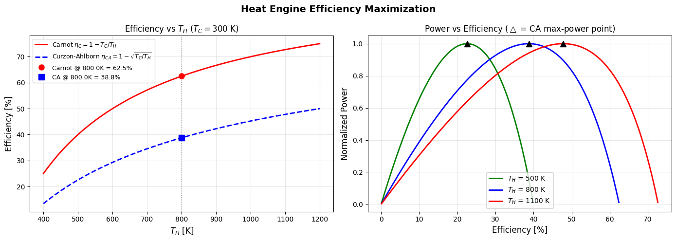
Figure 1 (2D): Efficiency vs $T_H$

The left panel shows both $\eta_C$ (red solid) and $\eta_{CA}$ (blue dashed) growing as $T_H$ increases, but $\eta_{CA}$ is always below $\eta_C$. The gap between them represents the cost of extracting finite power — you sacrifice some theoretical efficiency to get useful work out in finite time. At $T_H = 800$ K, Carnot gives 62.5% while CA gives only 38.7%, but the CA point delivers maximum power.

Figure 2 (2D): Power vs Efficiency (P-η curve)

Each colored curve shows how normalized power varies across the full efficiency range for a given $T_H$. The curves always peak (marked by black triangles ▲) at $\eta_{CA}$, then drop to zero as $\eta \to \eta_C$ (because the engine slows to a quasi-static crawl). This beautifully illustrates the efficiency-power tradeoff.

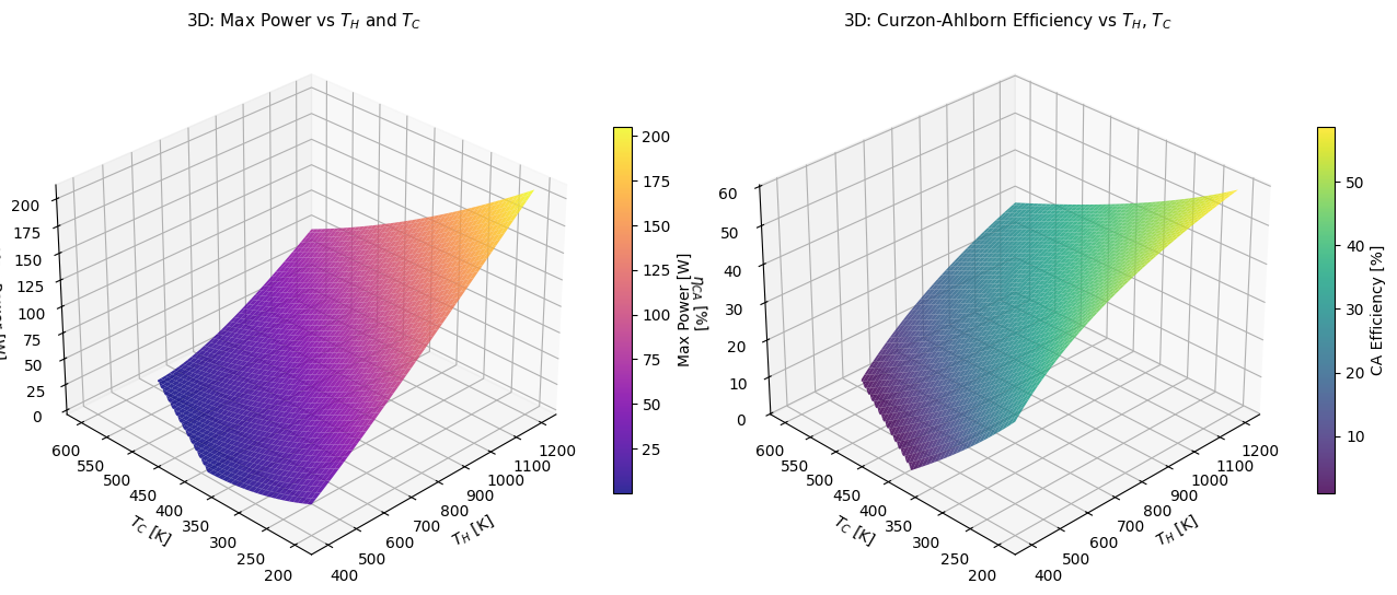
Figure 3 (3D): Power and CA Efficiency Surfaces

The left 3D surface shows $P_{max}(T_H, T_C)$ — power increases with larger temperature differences and higher $T_H$. The right surface shows $\eta_{CA}(T_H, T_C)$ — efficiency improves as $T_C$ drops or $T_H$ rises. Together they make clear that hot and cold extremes simultaneously maximize both power and efficiency, but in practice $T_C$ is set by the environment and $T_H$ is limited by materials.


Key Results from the Example ($T_H = 800$ K, $T_C = 300$ K)

Quantity Value
Carnot efficiency $\eta_C$ 62.50%
Curzon-Ahlborn efficiency $\eta_{CA}$ 38.73%
Maximum normalized power $P_{max}$ 0.1563 W
==================================================
Example: TH = 800.0 K, TC = 300.0 K
  Carnot efficiency       : 0.6250  (62.50%)
  Curzon-Ahlborn (max-P)  : 0.3876  (38.76%)
  Max power output (norm) : 78.1250 W
==================================================
  Numerical max-P at eta  : 0.3878  (38.78%)
  Analytical CA eta       : 0.3876


All plots saved.

The Curzon-Ahlborn efficiency is far more relevant to real engines than Carnot. For context, real coal power plants run at ~40% efficiency, which is remarkably close to $\eta_{CA}$ predictions — not $\eta_C$.


Takeaway

The condition for maximum power output from a heat engine with fixed $T_H$ and $T_C$ is to operate at the Curzon-Ahlborn efficiency $\eta_{CA} = 1 - \sqrt{T_C/T_H}$. This is the sweet spot between the two extremes: zero efficiency (short circuit) and Carnot efficiency (zero power). Real-world engine designers implicitly target this regime, which is why thermodynamic efficiency data from actual plants aligns so well with $\eta_{CA}$ rather than $\eta_C$.