Finding the Most Likely Distribution Under Constraints
Entropy maximization is one of the most elegant ideas in statistical mechanics and information theory. The core question is: given what we know, what probability distribution should we use? The answer: the one that maximizes entropy — the most “honest” or least biased distribution consistent with the constraints.
The Problem
Given a discrete random variable $X$ taking values ${x_1, x_2, \ldots, x_n}$ with probabilities ${p_1, p_2, \ldots, p_n}$, we want to maximize the Shannon entropy:
$$H(p) = -\sum_{i=1}^{n} p_i \log p_i$$
subject to constraints:
$$\sum_{i=1}^{n} p_i = 1 \quad \text{(normalization)}$$
$$\sum_{i=1}^{n} p_i \cdot x_i = \mu \quad \text{(mean constraint)}$$
$$\sum_{i=1}^{n} p_i \cdot x_i^2 = \mu^2 + \sigma^2 \quad \text{(variance constraint)}$$
Concrete Example
Suppose we have a die with faces ${1, 2, 3, 4, 5, 6}$. We observe:
- Mean: $\mu = 3.5$ (fair die average)
- Then add a twist: $\mu = 4.0$ (biased toward higher values)
We ask: what probability distribution maximizes entropy given this mean?
By the method of Lagrange multipliers, the solution takes the form of a Gibbs/Boltzmann distribution:
$$p_i^* = \frac{e^{\lambda x_i}}{Z(\lambda)}, \quad Z(\lambda) = \sum_{j} e^{\lambda x_j}$$
where $\lambda$ is chosen so that $\sum_i p_i x_i = \mu$.
Python Code
1 | import numpy as np |
Code Walkthrough
boltzmann_dist(lam, x) — computes $p_i = e^{\lambda x_i} / Z$ with the log-sum-exp trick (- np.max(...)) to avoid numerical overflow for large $|\lambda|$.
solve_lambda(mu_target, x) — the mean $\mathbb{E}[X]$ is a smooth, strictly monotone function of $\lambda$. Brent’s method (brentq) finds the unique root of $\mathbb{E}_\lambda[X] - \mu = 0$ in $O(\log(1/\varepsilon))$ iterations — much faster than gradient descent.
shannon_entropy(p) — uses scipy.special.entr which safely computes $-p \log p$ and returns 0 when $p = 0$.
Sweep over $\mu$ — we solve for $\lambda(\mu)$ at 400 values between the extremes, building a full picture of how the MaxEnt distribution changes with the constraint.
Graph Explanations
(a) Bar Chart shows the three distributions side-by-side. With $\mu = 3.5$, the MaxEnt solution is identical to the uniform — because no additional information is encoded beyond normalization. With $\mu = 4.0$, higher faces get larger probability, but the distribution is as spread out as possible given that constraint.
(b) H vs $\mu$ — entropy is maximized at $\mu = 3.5$ (the symmetric center of ${1,\ldots,6}$) and falls off toward the extremes where the distribution must concentrate mass. This curve is concave and symmetric around 3.5.
(c) $\lambda$ vs $\mu$ — $\lambda = 0$ corresponds to the uniform distribution ($\mu = 3.5$). Positive $\lambda$ tilts mass toward high faces; negative $\lambda$ toward low faces. The relationship is nonlinear and steeper near the extremes.
(d) 3-D Surface — the most visually rich panel. Each “slice” at a fixed $\mu$ is one MaxEnt distribution. You can see the probability mass shifting smoothly from low faces (left) to high faces (right) as $\mu$ increases from 1 to 6.
(e) Heatmap — same information as (d) but in 2-D. Bright regions = high probability. The diagonal bright band shows mass continuously tracking the constraint mean.
Key Takeaway
The MaxEnt principle says: use the distribution that is maximally noncommittal about everything you don’t know, while respecting everything you do know. When the only constraint is the mean, the answer is always a Gibbs/Boltzmann exponential family distribution — a result that bridges information theory, statistical mechanics, and Bayesian inference.
=== Fair-mean constraint (μ=3.5) ===
  P(X=1) = 0.166667
  P(X=2) = 0.166667
  P(X=3) = 0.166667
  P(X=4) = 0.166667
  P(X=5) = 0.166667
  P(X=6) = 0.166667
  λ = 0.000000,  H = 1.791759 nats

=== Biased-mean constraint (μ=4.0) ===
  P(X=1) = 0.103065
  P(X=2) = 0.122731
  P(X=3) = 0.146148
  P(X=4) = 0.174034
  P(X=5) = 0.207240
  P(X=6) = 0.246782
  λ = 0.174629,  H = 1.748506 nats

  Uniform entropy H = 1.791759 nats
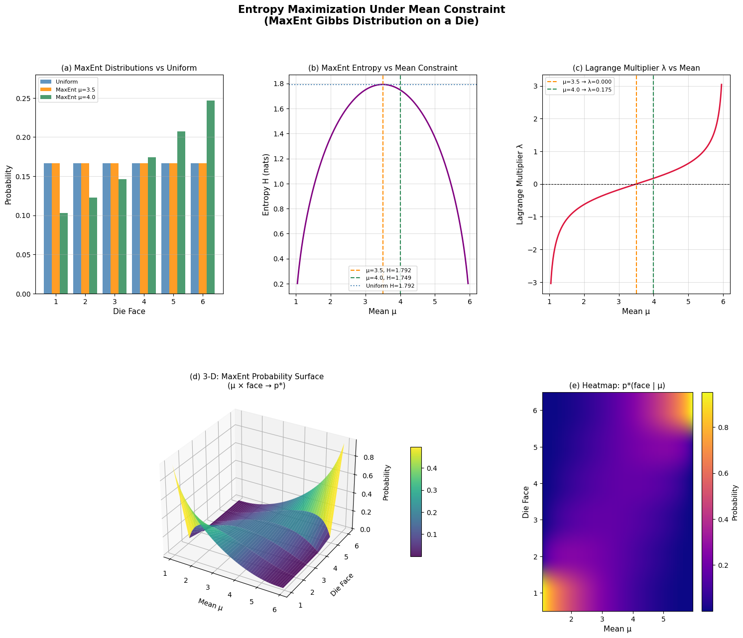
Figure saved.