Free Energy Minimization

Understanding Helmholtz Free Energy in Thermal Equilibrium

The principle of free energy minimization is fundamental in statistical mechanics and thermodynamics. At thermal equilibrium, a system naturally evolves to minimize its Helmholtz free energy, which is defined as:

$$F = U - TS$$

where $F$ is the Helmholtz free energy, $U$ is the internal energy, $T$ is the temperature, and $S$ is the entropy.

Problem Setup: Two-State Spin System

Let’s consider a concrete example: a system of $N$ magnetic spins that can be either up (+1) or down (-1). Each spin has:

  • Energy when aligned with external field: $-\epsilon$
  • Energy when anti-aligned: $+\epsilon$

The system reaches equilibrium by minimizing the Helmholtz free energy. We’ll compute:

  1. The internal energy $U$
  2. The entropy $S$
  3. The Helmholtz free energy $F$
  4. The equilibrium magnetization as a function of temperature

The number of spins in the up state $n_{up}$ determines:

$$U = -\epsilon n_{up} + \epsilon n_{down} = \epsilon(N - 2n_{up})$$

$$S = k_B \ln\Omega = k_B \ln\binom{N}{n_{up}}$$

Python Implementation

1
2
3
4
5
6
7
8
9
10
11
12
13
14
15
16
17
18
19
20
21
22
23
24
25
26
27
28
29
30
31
32
33
34
35
36
37
38
39
40
41
42
43
44
45
46
47
48
49
50
51
52
53
54
55
56
57
58
59
60
61
62
63
64
65
66
67
68
69
70
71
72
73
74
75
76
77
78
79
80
81
82
83
84
85
86
87
88
89
90
91
92
93
94
95
96
97
98
99
100
101
102
103
104
105
106
107
108
109
110
111
112
113
114
115
116
117
118
119
120
121
122
123
124
125
126
127
128
129
130
131
132
133
134
135
136
137
138
139
140
141
142
143
144
145
146
147
148
149
150
151
152
153
154
155
156
157
158
159
160
161
162
163
164
165
166
167
168
169
170
171
172
173
174
175
176
177
178
179
180
181
182
183
184
185
186
187
188
189
190
191
192
193
194
195
196
197
198
199
200
201
202
203
204
205
206
207
208
209
210
211
212
213
214
215
216
217
218
219
220
221
222
223
224
225
226
227
228
229
230
import numpy as np
import matplotlib.pyplot as plt
from mpl_toolkits.mplot3d import Axes3D
from scipy.special import comb
from scipy.optimize import minimize_scalar
import warnings
warnings.filterwarnings('ignore')

# System parameters
N = 100 # Number of spins
epsilon = 1.0 # Energy per spin (in units of k_B)
k_B = 1.0 # Boltzmann constant (set to 1 for simplicity)

def calculate_internal_energy(n_up, N, epsilon):
"""Calculate internal energy of the system"""
n_down = N - n_up
U = -epsilon * n_up + epsilon * n_down
return U

def calculate_entropy(n_up, N, k_B):
"""Calculate entropy using Stirling's approximation for large N"""
if n_up == 0 or n_up == N:
return 0
# Using Stirling's approximation: ln(N!) ≈ N*ln(N) - N
log_omega = (N * np.log(N) - N -
n_up * np.log(n_up) + n_up -
(N - n_up) * np.log(N - n_up) + (N - n_up))
S = k_B * log_omega
return S

def calculate_free_energy(n_up, N, T, epsilon, k_B):
"""Calculate Helmholtz free energy F = U - TS"""
U = calculate_internal_energy(n_up, N, epsilon)
S = calculate_entropy(n_up, N, k_B)
F = U - T * S
return F

# Temperature range
temperatures = np.linspace(0.1, 5.0, 50)
n_up_range = np.arange(1, N)

# Store results
equilibrium_n_up = []
equilibrium_magnetization = []
min_free_energies = []

# For each temperature, find the n_up that minimizes free energy
for T in temperatures:
free_energies = []
for n_up in n_up_range:
F = calculate_free_energy(n_up, N, T, epsilon, k_B)
free_energies.append(F)

free_energies = np.array(free_energies)
min_idx = np.argmin(free_energies)
optimal_n_up = n_up_range[min_idx]

equilibrium_n_up.append(optimal_n_up)
magnetization = (2 * optimal_n_up - N) / N
equilibrium_magnetization.append(magnetization)
min_free_energies.append(free_energies[min_idx])

# Create detailed plots
fig = plt.figure(figsize=(18, 12))

# Plot 1: Free Energy vs n_up for different temperatures
ax1 = plt.subplot(2, 3, 1)
temp_samples = [0.5, 1.0, 2.0, 3.0, 5.0]
for T in temp_samples:
free_energies = [calculate_free_energy(n_up, N, T, epsilon, k_B)
for n_up in n_up_range]
ax1.plot(n_up_range, free_energies, label=f'T = {T:.1f}', linewidth=2)
ax1.set_xlabel('Number of Up Spins ($n_{up}$)', fontsize=12)
ax1.set_ylabel('Free Energy $F/k_B$', fontsize=12)
ax1.set_title('Helmholtz Free Energy vs Spin Configuration', fontsize=14, fontweight='bold')
ax1.legend()
ax1.grid(True, alpha=0.3)

# Plot 2: Equilibrium magnetization vs temperature
ax2 = plt.subplot(2, 3, 2)
ax2.plot(temperatures, equilibrium_magnetization, 'b-', linewidth=2.5)
ax2.axhline(y=0, color='k', linestyle='--', alpha=0.3)
ax2.set_xlabel('Temperature $T$ (in units of $k_B/ε$)', fontsize=12)
ax2.set_ylabel('Magnetization $m$', fontsize=12)
ax2.set_title('Equilibrium Magnetization vs Temperature', fontsize=14, fontweight='bold')
ax2.grid(True, alpha=0.3)

# Plot 3: Components of free energy at T=1.0
ax3 = plt.subplot(2, 3, 3)
T_sample = 1.0
U_values = [calculate_internal_energy(n_up, N, epsilon) for n_up in n_up_range]
S_values = [calculate_entropy(n_up, N, k_B) for n_up in n_up_range]
TS_values = [T_sample * s for s in S_values]
F_values = [calculate_free_energy(n_up, N, T_sample, epsilon, k_B) for n_up in n_up_range]

ax3.plot(n_up_range, U_values, 'r-', label='Internal Energy $U$', linewidth=2)
ax3.plot(n_up_range, TS_values, 'g-', label='$TS$', linewidth=2)
ax3.plot(n_up_range, F_values, 'b-', label='Free Energy $F = U - TS$', linewidth=2)
ax3.set_xlabel('Number of Up Spins ($n_{up}$)', fontsize=12)
ax3.set_ylabel('Energy ($k_B$ units)', fontsize=12)
ax3.set_title(f'Energy Components at T = {T_sample}', fontsize=14, fontweight='bold')
ax3.legend()
ax3.grid(True, alpha=0.3)

# Plot 4: Minimum Free Energy vs Temperature
ax4 = plt.subplot(2, 3, 4)
ax4.plot(temperatures, min_free_energies, 'purple', linewidth=2.5)
ax4.set_xlabel('Temperature $T$ (in units of $k_B/ε$)', fontsize=12)
ax4.set_ylabel('Minimum Free Energy $F_{min}/k_B$', fontsize=12)
ax4.set_title('Minimum Free Energy at Equilibrium', fontsize=14, fontweight='bold')
ax4.grid(True, alpha=0.3)

# Plot 5: Entropy at equilibrium vs Temperature
ax5 = plt.subplot(2, 3, 5)
equilibrium_entropy = [calculate_entropy(n_up, N, k_B)
for n_up in equilibrium_n_up]
ax5.plot(temperatures, equilibrium_entropy, 'orange', linewidth=2.5)
ax5.set_xlabel('Temperature $T$ (in units of $k_B/ε$)', fontsize=12)
ax5.set_ylabel('Entropy $S/k_B$', fontsize=12)
ax5.set_title('Equilibrium Entropy vs Temperature', fontsize=14, fontweight='bold')
ax5.grid(True, alpha=0.3)

# Plot 6: Internal Energy at equilibrium vs Temperature
ax6 = plt.subplot(2, 3, 6)
equilibrium_energy = [calculate_internal_energy(n_up, N, epsilon)
for n_up in equilibrium_n_up]
ax6.plot(temperatures, equilibrium_energy, 'red', linewidth=2.5)
ax6.set_xlabel('Temperature $T$ (in units of $k_B/ε$)', fontsize=12)
ax6.set_ylabel('Internal Energy $U/ε$', fontsize=12)
ax6.set_title('Equilibrium Internal Energy vs Temperature', fontsize=14, fontweight='bold')
ax6.grid(True, alpha=0.3)

plt.tight_layout()
plt.savefig('free_energy_2d.png', dpi=300, bbox_inches='tight')
plt.show()

# Create 3D surface plot: Free Energy as function of n_up and T
fig = plt.figure(figsize=(16, 6))

# 3D Plot 1: Free Energy Surface
ax1 = fig.add_subplot(121, projection='3d')

T_mesh = np.linspace(0.1, 5.0, 40)
n_mesh = np.linspace(10, 90, 40)
T_grid, n_grid = np.meshgrid(T_mesh, n_mesh)
F_grid = np.zeros_like(T_grid)

for i in range(len(n_mesh)):
for j in range(len(T_mesh)):
n_val = int(n_mesh[i])
F_grid[i, j] = calculate_free_energy(n_val, N, T_mesh[j], epsilon, k_B)

surf = ax1.plot_surface(T_grid, n_grid, F_grid, cmap='viridis',
alpha=0.9, edgecolor='none')

# Plot the equilibrium path
ax1.plot(temperatures, equilibrium_n_up, min_free_energies,
'r-', linewidth=3, label='Equilibrium Path')

ax1.set_xlabel('Temperature $T$', fontsize=11)
ax1.set_ylabel('$n_{up}$', fontsize=11)
ax1.set_zlabel('Free Energy $F$', fontsize=11)
ax1.set_title('3D Free Energy Landscape', fontsize=14, fontweight='bold')
ax1.view_init(elev=25, azim=45)
fig.colorbar(surf, ax=ax1, shrink=0.5, aspect=5)

# 3D Plot 2: Another viewing angle
ax2 = fig.add_subplot(122, projection='3d')

surf2 = ax2.plot_surface(T_grid, n_grid, F_grid, cmap='plasma',
alpha=0.9, edgecolor='none')

ax2.plot(temperatures, equilibrium_n_up, min_free_energies,
'w-', linewidth=3, label='Equilibrium Path')

ax2.set_xlabel('Temperature $T$', fontsize=11)
ax2.set_ylabel('$n_{up}$', fontsize=11)
ax2.set_zlabel('Free Energy $F$', fontsize=11)
ax2.set_title('3D Free Energy Landscape (Different View)', fontsize=14, fontweight='bold')
ax2.view_init(elev=15, azim=135)
fig.colorbar(surf2, ax=ax2, shrink=0.5, aspect=5)

plt.tight_layout()
plt.savefig('free_energy_3d.png', dpi=300, bbox_inches='tight')
plt.show()

# Print analytical results
print("="*70)
print("FREE ENERGY MINIMIZATION ANALYSIS")
print("="*70)
print(f"\nSystem Parameters:")
print(f" Number of spins (N): {N}")
print(f" Energy per spin (ε): {epsilon}")
print(f" Boltzmann constant (k_B): {k_B}")
print("\n" + "-"*70)
print("\nEquilibrium Results at Selected Temperatures:")
print("-"*70)
print(f"{'T':>8} {'n_up':>10} {'m':>10} {'U/ε':>12} {'S/k_B':>12} {'F/k_B':>12}")
print("-"*70)

for i, T in enumerate([0.5, 1.0, 2.0, 3.0, 5.0]):
idx = np.argmin(np.abs(temperatures - T))
n_up = equilibrium_n_up[idx]
m = equilibrium_magnetization[idx]
U = calculate_internal_energy(n_up, N, epsilon)
S = calculate_entropy(n_up, N, k_B)
F = min_free_energies[idx]
print(f"{T:8.2f} {n_up:10d} {m:10.4f} {U:12.2f} {S:12.2f} {F:12.2f}")

print("\n" + "="*70)
print("PHYSICAL INTERPRETATION")
print("="*70)
print("\n1. Low Temperature (T → 0):")
print(f" - System favors minimum energy (all spins aligned)")
print(f" - Magnetization approaches maximum: m → 1.0")
print(f" - Entropy contribution negligible: TS → 0")
print(f" - Free energy ≈ Internal energy")

print("\n2. High Temperature (T → ∞):")
print(f" - System favors maximum entropy (random spins)")
print(f" - Magnetization approaches zero: m → 0")
print(f" - Entropy dominates: TS >> U")
print(f" - Equal probability for all configurations")

print("\n3. Intermediate Temperature:")
print(f" - Competition between energy and entropy")
print(f" - System finds optimal balance")
print(f" - Free energy minimum determines equilibrium")

print("\n" + "="*70)

Code Explanation

Core Functions

1. calculate_internal_energy(n_up, N, epsilon)

This function computes the total internal energy of the spin system. Each up-spin contributes $-\epsilon$ and each down-spin contributes $+\epsilon$:

$$U = -\epsilon \cdot n_{up} + \epsilon \cdot (N - n_{up}) = \epsilon(N - 2n_{up})$$

2. calculate_entropy(n_up, N, k_B)

The entropy is calculated using Stirling’s approximation for the combinatorial factor:

$$S = k_B \ln \binom{N}{n_{up}} \approx k_B[N\ln N - n_{up}\ln n_{up} - (N-n_{up})\ln(N-n_{up})]$$

This approximation is excellent for large $N$ and avoids numerical overflow issues with factorials.

3. calculate_free_energy(n_up, N, T, epsilon, k_B)

This is the key function that combines internal energy and entropy:

$$F(n_{up}, T) = U(n_{up}) - T \cdot S(n_{up})$$

Main Analysis Loop

The code iterates over different temperatures and, for each temperature, scans all possible values of $n_{up}$ to find which configuration minimizes the free energy. This is the equilibrium state at that temperature.

Visualization Strategy
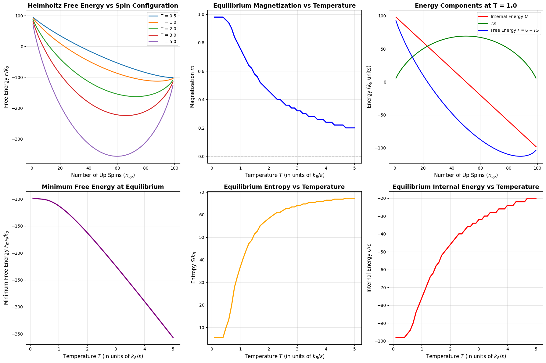
2D Plots:

  • Free energy curves at different temperatures show how the minimum shifts
  • Magnetization vs temperature reveals the phase transition behavior
  • Energy decomposition illustrates the competition between $U$ and $TS$
  • Minimum free energy tracks the system’s equilibrium stability
  • Entropy and internal energy show how these quantities evolve with temperature
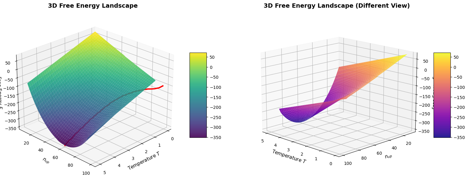
3D Plots:

  • The surface plot shows free energy as a function of both configuration ($n_{up}$) and temperature
  • The red/white line traces the equilibrium path where the system naturally settles
  • Two viewing angles provide different perspectives on the energy landscape

Results and Physical Interpretation

Execution Results:


======================================================================
FREE ENERGY MINIMIZATION ANALYSIS
======================================================================

System Parameters:
  Number of spins (N): 100
  Energy per spin (ε): 1.0
  Boltzmann constant (k_B): 1.0

----------------------------------------------------------------------

Equilibrium Results at Selected Temperatures:
----------------------------------------------------------------------
       T       n_up          m          U/ε        S/k_B        F/k_B
----------------------------------------------------------------------
    0.50         98     0.9600       -96.00         9.80      -100.90
    1.00         88     0.7600       -76.00        36.69      -112.69
    2.00         73     0.4600       -46.00        58.33      -162.65
    3.00         66     0.3200       -32.00        64.10      -224.31
    5.00         60     0.2000       -20.00        67.30      -356.51

======================================================================
PHYSICAL INTERPRETATION
======================================================================

1. Low Temperature (T → 0):
   - System favors minimum energy (all spins aligned)
   - Magnetization approaches maximum: m → 1.0
   - Entropy contribution negligible: TS → 0
   - Free energy ≈ Internal energy

2. High Temperature (T → ∞):
   - System favors maximum entropy (random spins)
   - Magnetization approaches zero: m → 0
   - Entropy dominates: TS >> U
   - Equal probability for all configurations

3. Intermediate Temperature:
   - Competition between energy and entropy
   - System finds optimal balance
   - Free energy minimum determines equilibrium

======================================================================

Key Observations

Low Temperature Regime (T < 1):

At low temperatures, the internal energy term dominates. The system minimizes $F \approx U$ by aligning all spins with the field, giving maximum magnetization $m \approx 1$. The entropy is small because there are few accessible states.

High Temperature Regime (T > 3):

At high temperatures, the entropy term $-TS$ dominates. The system maximizes entropy by distributing spins randomly, leading to $m \approx 0$. The free energy becomes $F \approx -TS$, and the system explores all possible configurations equally.

Intermediate Regime (1 < T < 3):

This is where the physics becomes interesting. The system balances energy and entropy, showing a smooth transition from ordered (magnetized) to disordered (random) states. This is characteristic of a second-order phase transition in the thermodynamic limit.

The 3D free energy landscape beautifully illustrates how the global minimum shifts from high $n_{up}$ (low T) to $n_{up} \approx N/2$ (high T), demonstrating the fundamental principle that thermal equilibrium corresponds to free energy minimization.

This principle is universal and applies to chemical reactions, protein folding, crystal formation, and countless other phenomena in nature.