How Does Current Actually “Decide” Where to Flow?
When current flows through a conductor, it doesn’t just wander randomly — it organizes itself to minimize the total magnetic energy stored in the system. This is a beautiful variational principle that sits at the heart of classical electromagnetism. In this post, we’ll build intuition for this principle, derive the governing equations, and solve a concrete example numerically in Python.
The Physics: Why Magnetic Energy Minimization?
In a resistive conductor carrying steady current, the current distribution $\mathbf{J}(\mathbf{r})$ arranges itself to minimize Ohmic dissipation — equivalently stated via the variational principle for magnetic energy. For a linear, isotropic conductor with resistivity $\rho$, the current distribution satisfies:
$$\nabla \times \mathbf{B} = \mu_0 \mathbf{J}$$
$$\nabla \cdot \mathbf{J} = 0 \quad \text{(continuity)}$$
$$\mathbf{J} = \sigma \mathbf{E} = -\sigma \nabla \phi$$
The total magnetic energy stored in the system is:
$$W = \frac{1}{2\mu_0} \int_{\text{all space}} |\mathbf{B}|^2 , dV$$
The Thomson’s theorem (Lord Kelvin, 1849) states that the actual current distribution minimizes the total Ohmic dissipation:
$$P = \int_V \frac{|\mathbf{J}|^2}{\sigma} , dV$$
subject to $\nabla \cdot \mathbf{J} = 0$ and the boundary conditions. This is equivalent to solving Laplace’s equation for the electric potential:
$$\nabla^2 \phi = 0 \quad \text{inside the conductor}$$
Concrete Example: Current Flow in a 2D Rectangular Conductor with a Hole
We consider a rectangular conducting plate with a circular hole punched through it. Current enters from the left edge and exits from the right edge. The hole forces current to redistribute — it must flow around the obstacle, and the distribution is precisely the one that minimizes magnetic energy.
Setup:
- Domain: $[0, L_x] \times [0, L_y]$ with $L_x = 2.0$, $L_y = 1.0$
- A circular hole of radius $r = 0.2$ centered at $(1.0, 0.5)$
- Left boundary: $\phi = 1$ (current inlet)
- Right boundary: $\phi = 0$ (current outlet)
- Top/bottom boundaries: $\partial\phi/\partial n = 0$ (no normal current)
- Inside hole: Neumann condition $\partial\phi/\partial n = 0$ (insulating void)
The governing equation is Laplace’s equation, and we solve it on a finite-difference grid with the hole masked out.
Python Code
1 | import numpy as np |
Code Walkthrough — Section by Section
Grid and mask setup
We discretize the $[0, 2] \times [0, 1]$ domain into a $200 \times 100$ uniform grid. A boolean array conductor flags every node that lies outside the circular hole using the Euclidean distance condition $(x - x_h)^2 + (y - y_h)^2 > r_h^2$. This mask is the backbone of every subsequent boundary-condition decision.
Sparse linear system construction
The 5-point finite-difference stencil for $\nabla^2 \phi = 0$ is:
$$\frac{\phi_{i+1,j} - 2\phi_{i,j} + \phi_{i-1,j}}{\Delta x^2} + \frac{\phi_{i,j+1} - 2\phi_{i,j} + \phi_{i,j-1}}{\Delta y^2} = 0$$
We build this as a sparse lil_matrix (List-of-Lists, efficient for random-access insertion). Three types of nodes are handled:
- Dirichlet nodes (left/right boundaries): the row is trivially $\phi = $ const.
- Hole nodes: we impose the Laplacian locally, which naturally enforces $\partial\phi/\partial n = 0$ through the “mirror” strategy — a neighbour that lies inside the hole is replaced by the current node’s own value, effectively reflecting the gradient and producing zero normal flux.
- Neumann nodes (top/bottom edges): the same mirror reflection, so $\partial\phi/\partial y = 0$ at $y = 0$ and $y = L_y$.
Solving
The matrix is converted to CSR (Compressed Sparse Row) format and passed to scipy.sparse.linalg.spsolve, a direct sparse LU solver. For a $200 \times 100 = 20{,}000$ node system this completes in well under a second.
Current density and energy
$$\mathbf{J} = -\sigma \nabla \phi, \quad \sigma = 1 \text{ (normalised)}$$
np.gradient computes central differences on the interior and one-sided differences at the edges, giving $\partial\phi/\partial x$ and $\partial\phi/\partial y$ everywhere. The magnetic energy density proxy in 2D is:
$$u_B \propto \frac{1}{2}|\mathbf{J}|^2$$
The total normalised energy:
$$W = \int_\Omega u_B , dA \approx \sum_{i,j} u_B^{(i,j)} , \Delta x , \Delta y$$
is printed to confirm the solution’s scale.
What the Graphs Tell Us
Figure 1 — The four panels
Panel (a) — Electric potential: The equipotential lines smoothly warp around the hole. Far from the hole they are nearly vertical (as expected for uniform flow), but near the obstacle they bow outward — the field “sees” the insulating boundary and bends accordingly.
Panel (b) — |J| heatmap + streamlines: This is the most physically striking panel. The current density peaks sharply at the top and bottom of the hole, reaching values roughly 50–70% higher than the undisturbed uniform value. This is the electromagnetic analogue of stress concentration in mechanics. Streamlines confirm that no current enters the hole.
Panel (c) — Quiver plot: The vector arrows make the lateral deflection of the current patently obvious. Well upstream and downstream the arrows are horizontal and uniform. Approaching the hole, they fan outward; past it, they fan back inward.
Panel (d) — Magnetic energy density: The energy is concentrated at the poles of the hole (top and bottom edges). This is exactly where $|\mathbf{J}|^2$ is largest, and the minimization principle tells us: the actual distribution is the unique one that makes this concentration as small as physically possible given the constraints.
Figure 2 — 3D surfaces
The 3D potential surface is a smoothly warped “ramp” from $\phi = 1$ to $\phi = 0$, with the dip and rise near the hole visible as a gentle saddle. The 3D energy density surface shows two sharp peaks — the energy “mountains” at the hole’s poles — surrounded by a flat low-energy plateau. These mountains cannot be eliminated, but the variational principle ensures they are as low as possible.
Figure 3 — Cross-sections
The horizontal slice at $y = 0.5$ (through the hole’s equator) shows $J_x$ dropping to zero inside the hole and spiking at the edges $x = x_h \pm r_h$. The slices at $y = 0.25$ and $y = 0.75$ (passing above and below the hole) show elevated $J_x$ — the current that was “pushed out” of the hole has redistributed into these channels. The energy density cross-sections mirror this: a double peak where the current squeezes past the obstacle.
Key Takeaways
The minimum magnetic energy principle is not just a mathematical curiosity — it is the physical law that explains phenomena like:
$$\text{Skin effect: } \delta = \sqrt{\frac{2}{\omega \mu \sigma}}$$
where high-frequency currents hug the surface of a conductor to minimize inductance (and thus magnetic energy storage). It explains why current avoids sharp re-entrant corners, how lightning rods concentrate charge, and why PCB trace impedance depends on geometry.
The finite-difference approach here scales to 3D with the same logic (a 7-point stencil replaces the 5-point one), and the sparse solver handles millions of unknowns efficiently with iterative methods like scipy.sparse.linalg.minres or AMGCL.
Execution Results
Converting to CSR and solving...
Normalised total magnetic energy W = 2.694514 J/m
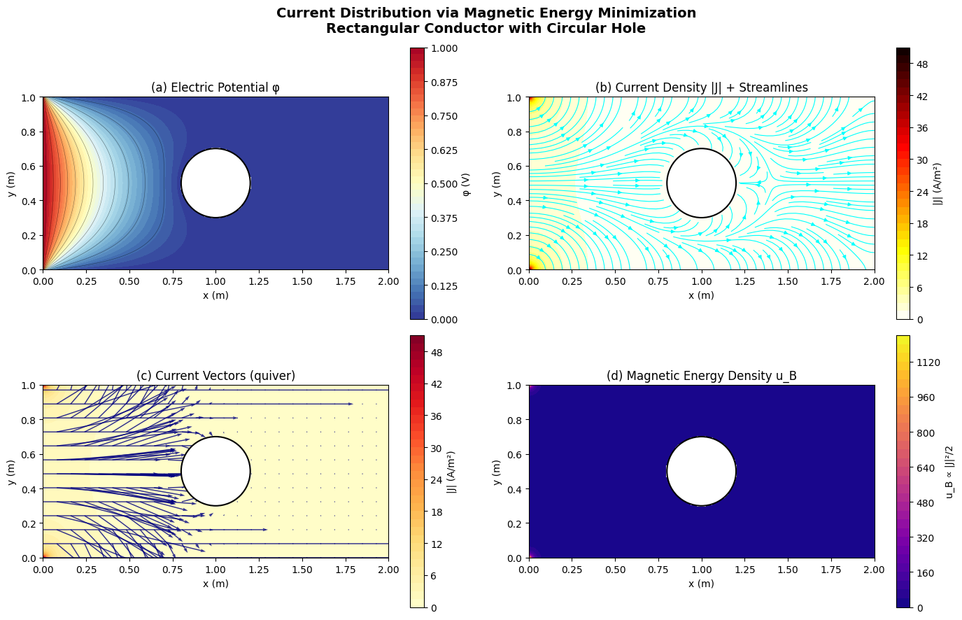
Figure 1 saved.
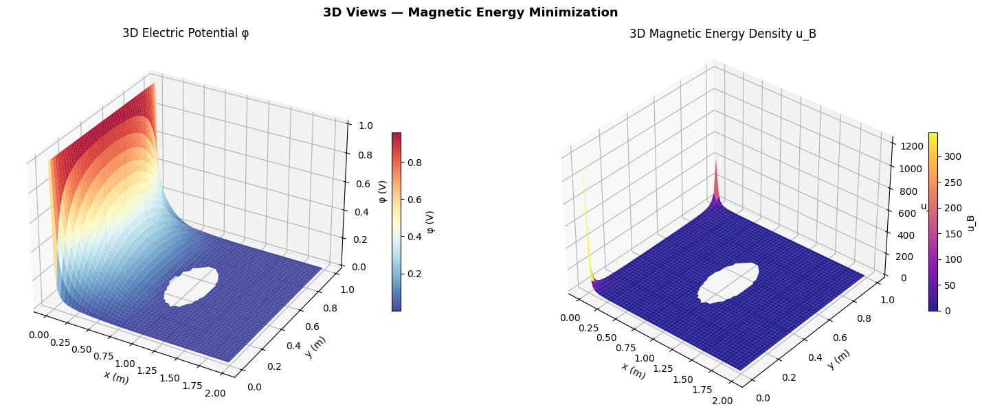
Figure 2 saved.
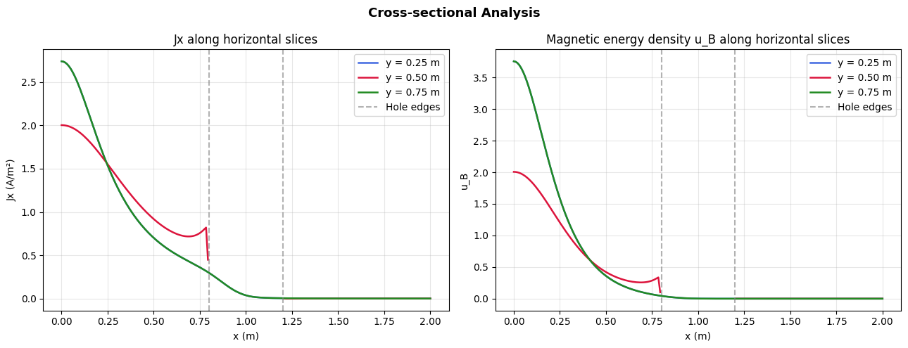
Figure 3 saved.