Optimizing Charge Distribution on Conductor Surfaces

Minimizing Energy Under Constant Potential

Introduction

One of the most elegant problems in electrostatics is this: given a conductor held at a fixed potential, what charge distribution on its surface minimizes the electrostatic energy?

The answer, grounded in variational principles, is that the physical equilibrium distribution is exactly the energy-minimizing one — nature solves an optimization problem every time charges settle on a conductor.

In this post, we’ll walk through the mathematics, set up a concrete numerical example (a 2D conducting ring and a 3D conducting sphere), and solve everything in Python.


Mathematical Framework

Energy of a Charge Distribution

The electrostatic energy of a surface charge distribution $\sigma(\mathbf{r})$ is:

$$W = \frac{1}{2} \iint \iint \frac{\sigma(\mathbf{r}), \sigma(\mathbf{r}’)}{4\pi\varepsilon_0 |\mathbf{r} - \mathbf{r}’|} , dS, dS’$$

The Constraint

The conductor surface is held at a fixed potential $V_0$. The potential at any surface point must equal $V_0$:

$$\phi(\mathbf{r}) = \frac{1}{4\pi\varepsilon_0} \int \frac{\sigma(\mathbf{r}’)}{|\mathbf{r} - \mathbf{r}’|} , dS’ = V_0 \quad \forall, \mathbf{r} \in S$$

Variational Condition

Using a Lagrange multiplier $\lambda$ for the total charge $Q = \int \sigma, dS$, minimizing:

$$\delta\left[ W - \lambda \int \sigma, dS \right] = 0$$

yields the integral equation:

$$\frac{1}{4\pi\varepsilon_0} \int \frac{\sigma(\mathbf{r}’)}{|\mathbf{r} - \mathbf{r}’|} , dS’ = \lambda$$

This is precisely the constant-potential condition. The Lagrange multiplier is identified as $\lambda = V_0$, confirming that the equilibrium charge distribution is the energy minimizer.

Discretized Form

Dividing the surface into $N$ elements with charges $q_i$, the energy is:

$$W = \frac{1}{2} \mathbf{q}^T \mathbf{P} \mathbf{q}$$

where $P_{ij} = \dfrac{1}{4\pi\varepsilon_0 r_{ij}}$ is the Maxwell elastance matrix. The potential condition becomes:

$$\mathbf{P} \mathbf{q} = V_0 \mathbf{1}$$

Solving this linear system gives the optimal charge distribution.


Concrete Examples

We solve two cases:

  • 2D ring conductor: $N$ point charges arranged on a circle of radius $R$
  • 3D sphere conductor: charges distributed on a spherical surface

For the 3D sphere, the analytical answer is known — $\sigma = \text{const}$ — which gives us a perfect verification target.


Python Source Code

1
2
3
4
5
6
7
8
9
10
11
12
13
14
15
16
17
18
19
20
21
22
23
24
25
26
27
28
29
30
31
32
33
34
35
36
37
38
39
40
41
42
43
44
45
46
47
48
49
50
51
52
53
54
55
56
57
58
59
60
61
62
63
64
65
66
67
68
69
70
71
72
73
74
75
76
77
78
79
80
81
82
83
84
85
86
87
88
89
90
91
92
93
94
95
96
97
98
99
100
101
102
103
104
105
106
107
108
109
110
111
112
113
114
115
116
117
118
119
120
121
122
123
124
125
126
127
128
129
130
131
132
133
134
135
136
137
138
139
140
141
142
143
144
145
146
147
148
149
150
151
152
153
154
155
156
157
158
159
160
161
162
163
164
165
166
167
168
169
170
171
172
173
174
175
176
177
178
179
180
181
182
183
184
185
186
187
188
189
190
191
192
193
194
195
196
197
198
199
200
201
202
203
204
205
206
207
208
209
210
211
212
213
214
215
216
217
218
219
220
221
222
223
224
225
226
227
228
229
230
231
232
233
234
235
236
237
238
239
240
241
242
243
244
245
246
247
248
249
250
251
252
253
254
255
256
257
258
259
260
261
262
263
264
265
266
267
268
269
270
271
272
273
274
275
276
277
278
279
280
281
282
283
284
285
286
287
288
289
290
291
292
293
294
295
296
297
298
299
300
301
302
303
304
305
306
307
308
309
310
311
312
313
314
315
316
317
318
319
320
321
322
323
324
325
326
327
328
329
330
331
332
333
334
335
336
337
338
339
340
341
342
343
344
345
346
347
348
349
350
351
352
353
354
355
356
357
358
359
360
361
362
363
364
365
366
367
368
369
370
371
372
373
374
375
376
377
378
379
380
381
382
383
384
385
386
387
388
389
390
391
392
393
394
395
396
397
398
399
400
401
402
403
404
405
406
407
408
409
410
411
412
413
414
415
416
417
418
419
420
421
422
423
424
425
426
427
428
429
430
431
432
433
434
435
"""
============================================================
Optimizing Charge Distribution on Conductor Surfaces
Minimizing Electrostatic Energy Under Constant Potential
============================================================
"""

# ── Imports ──────────────────────────────────────────────
import numpy as np
import matplotlib.pyplot as plt
import matplotlib.gridspec as gridspec
from mpl_toolkits.mplot3d import Axes3D
from scipy.spatial.distance import cdist
import warnings
warnings.filterwarnings('ignore')

# ── Physical Constants ────────────────────────────────────
EPS0 = 8.854187817e-12 # permittivity of free space [F/m]
K_E = 1.0 / (4 * np.pi * EPS0) # Coulomb constant [N·m²/C²]
V0 = 1.0 # target potential [V]
R = 1.0 # conductor radius [m]

# =============================================================
# PART 1: 2D Ring Conductor
# =============================================================

def build_elastance_2d(N, R, reg=1e-2):
"""
Build the Maxwell elastance matrix P for N point charges on a 2D ring.

For i != j : P_ij = K_E / r_ij (Coulomb interaction)
For i == j : P_ii = K_E / a_self (self-energy regularisation)
"""
theta = np.linspace(0, 2 * np.pi, N, endpoint=False)
x = R * np.cos(theta)
y = R * np.sin(theta)

pos = np.stack([x, y], axis=1) # (N, 2)
D = cdist(pos, pos) # pairwise distances (N, N)

P = np.zeros((N, N))
off = np.where(D > 0)
P[off] = K_E / D[off]

# Self-energy: treat each element as a disc of radius a = sqrt(πR²/N)
a_self = np.sqrt(np.pi * R**2 / N)
np.fill_diagonal(P, K_E / a_self)

return P, x, y


def solve_charge_distribution_2d(N=64, R=1.0, V0=1.0):
"""
Solve P q = V0 * ones for the 2D ring.
Returns q (charges), positions, energy W.
"""
P, x, y = build_elastance_2d(N, R)
rhs = V0 * np.ones(N)
q = np.linalg.solve(P, rhs)
W = 0.5 * q @ P @ q
return q, x, y, W, P


# =============================================================
# PART 2: 3D Sphere Conductor (using Fibonacci lattice)
# =============================================================

def fibonacci_sphere(N):
"""
Generate N near-uniformly distributed points on the unit sphere
using the Fibonacci / golden-ratio lattice.
"""
phi = np.pi * (3.0 - np.sqrt(5.0)) # golden angle [rad]
idx = np.arange(N)
z_arr = 1.0 - (2.0 * idx + 1.0) / N
r_arr = np.sqrt(np.maximum(1.0 - z_arr**2, 0.0))
theta = phi * idx
x_arr = r_arr * np.cos(theta)
y_arr = r_arr * np.sin(theta)
return x_arr, y_arr, z_arr


def build_elastance_3d(N, R):
"""
Build the elastance matrix for N points on a sphere of radius R.
Self-energy: a = 2R / sqrt(N) (Wigner-Seitz estimate)
"""
x, y, z = fibonacci_sphere(N)
x, y, z = R * x, R * y, R * z

pos = np.stack([x, y, z], axis=1) # (N, 3)
D = cdist(pos, pos) # (N, N)

P = np.zeros((N, N))
off = np.where(D > 0)
P[off] = K_E / D[off]

a_self = 2.0 * R / np.sqrt(N)
np.fill_diagonal(P, K_E / a_self)

return P, x, y, z


def solve_charge_distribution_3d(N=300, R=1.0, V0=1.0):
"""
Solve P q = V0 * ones for the 3D sphere.
Uses np.linalg.lstsq for numerical stability.
"""
P, x, y, z = build_elastance_3d(N, R)
rhs = V0 * np.ones(N)
q, *_ = np.linalg.lstsq(P, rhs, rcond=None)
W = 0.5 * q @ P @ q
return q, x, y, z, W, P


# =============================================================
# PART 3: Verify Energy Minimum via Perturbation Test
# =============================================================

def perturbation_energy_test(q_opt, P, n_trials=200, epsilon=0.05):
"""
Randomly perturb q_opt (keeping total charge fixed) and confirm
all perturbed energies >= W_opt.
"""
W_opt = 0.5 * q_opt @ P @ q_opt
N = len(q_opt)
W_perturbed = np.empty(n_trials)

rng = np.random.default_rng(42)
for i in range(n_trials):
dq = rng.standard_normal(N)
dq -= dq.mean() # enforce Σδq = 0
dq *= epsilon * np.linalg.norm(q_opt) / np.linalg.norm(dq)
q_new = q_opt + dq
W_perturbed[i] = 0.5 * q_new @ P @ q_new

return W_opt, W_perturbed


# =============================================================
# PART 4: Potential Map around the 2D Ring
# =============================================================

def compute_potential_map_2d(q, x_src, y_src, grid_res=200, extent=2.5):
"""
Compute the electrostatic potential on a 2D grid.
"""
gx = np.linspace(-extent, extent, grid_res)
gy = np.linspace(-extent, extent, grid_res)
GX, GY = np.meshgrid(gx, gy)
PHI = np.zeros_like(GX)

for i in range(len(q)):
dx = GX - x_src[i]
dy = GY - y_src[i]
dist = np.sqrt(dx**2 + dy**2)
dist = np.maximum(dist, R / 10)
PHI += K_E * q[i] / dist

return GX, GY, PHI


# =============================================================
# MAIN COMPUTATION
# =============================================================

print("=" * 60)
print(" Charge Distribution Optimisation on Conductors")
print("=" * 60)

N2D = 80
N3D = 400

print(f"\n[2D] Solving ring conductor (N = {N2D}) ...")
q2d, x2d, y2d, W2d, P2d = solve_charge_distribution_2d(N2D, R, V0)
print(f" Total charge Q = {q2d.sum():.6e} C")
print(f" Energy W = {W2d:.6e} J")

phi_check = P2d @ q2d
print(f" Potential min/max = {phi_check.min():.4f} / {phi_check.max():.4f} (target {V0})")

print(f"\n[3D] Solving sphere conductor (N = {N3D}) ...")
q3d, x3d, y3d, z3d, W3d, P3d = solve_charge_distribution_3d(N3D, R, V0)
print(f" Total charge Q = {q3d.sum():.6e} C")
print(f" Energy W = {W3d:.6e} J")

phi_check3 = P3d @ q3d
print(f" Potential min/max = {phi_check3.min():.4f} / {phi_check3.max():.4f} (target {V0})")

print("\n[2D] Running perturbation test ...")
W_opt2d, W_pert2d = perturbation_energy_test(q2d, P2d, n_trials=300)
print(f" W_opt = {W_opt2d:.6e} | all perturbed >= W_opt : {np.all(W_pert2d >= W_opt2d - 1e-10)}")

print("\n[2D] Computing potential map ...")
GX, GY, PHI = compute_potential_map_2d(q2d, x2d, y2d, grid_res=300)

print("\nAll computation complete. Generating plots ...")


# =============================================================
# PART 5: VISUALISATION
# =============================================================

plt.rcParams.update({
'font.family' : 'DejaVu Sans',
'font.size' : 11,
'axes.titlesize': 13,
'axes.labelsize': 11,
'figure.facecolor': '#0d1117',
'axes.facecolor' : '#161b22',
'text.color' : '#e6edf3',
'axes.labelcolor' : '#e6edf3',
'xtick.color' : '#8b949e',
'ytick.color' : '#8b949e',
'axes.edgecolor' : '#30363d',
'grid.color' : '#21262d',
'grid.linewidth' : 0.5,
})
ACCENT = '#58a6ff'
ACCENT2 = '#f78166'
ACCENT3 = '#3fb950'

fig = plt.figure(figsize=(20, 22))
fig.patch.set_facecolor('#0d1117')

gs = gridspec.GridSpec(
3, 3,
figure=fig,
hspace=0.42,
wspace=0.38,
top=0.93, bottom=0.05,
left=0.07, right=0.97
)

fig.suptitle(
'Charge Distribution Optimisation on Conductor Surfaces\n'
r'Minimising $W = \frac{1}{2}\,\mathbf{q}^T\mathbf{P}\mathbf{q}$ '
r'subject to $\mathbf{P}\mathbf{q} = V_0\,\mathbf{1}$',
fontsize=14, color='#e6edf3', y=0.97
)

theta_2d = np.linspace(0, 2 * np.pi, N2D, endpoint=False)

# ── Plot 1: 2D ring charge distribution ──────────────────
ax1 = fig.add_subplot(gs[0, 0])
scatter = ax1.scatter(x2d, y2d, c=q2d, cmap='plasma', s=60,
vmin=q2d.min(), vmax=q2d.max(),
zorder=3, edgecolors='none')
circle = plt.Circle((0, 0), R, color=ACCENT, fill=False,
linestyle='--', linewidth=1, alpha=0.4)
ax1.add_patch(circle)
cb1 = plt.colorbar(scatter, ax=ax1, pad=0.02)
cb1.set_label('Charge $q_i$ [C]', color='#e6edf3')
cb1.ax.yaxis.set_tick_params(color='#8b949e')
ax1.set_aspect('equal')
ax1.set_title('2D Ring: Charge per Element', color='#e6edf3')
ax1.set_xlabel('$x$ [m]')
ax1.set_ylabel('$y$ [m]')
ax1.grid(True, alpha=0.3)
ax1.set_xlim(-1.5, 1.5)
ax1.set_ylim(-1.5, 1.5)

# ── Plot 2: Charge vs angle ───────────────────────────────
ax2 = fig.add_subplot(gs[0, 1])
ax2.plot(np.degrees(theta_2d), q2d, color=ACCENT, linewidth=2, label='Numerical')
ax2.axhline(q2d.mean(), color=ACCENT2, linewidth=1.5,
linestyle='--', label=f'Mean = {q2d.mean():.2e} C')
ax2.fill_between(np.degrees(theta_2d), q2d.mean(), q2d, alpha=0.25, color=ACCENT)
ax2.set_title('2D Ring: $q_i$ vs Angle', color='#e6edf3')
ax2.set_xlabel('Angle $\\theta$ [°]')
ax2.set_ylabel('Charge $q_i$ [C]')
ax2.legend(loc='upper right', fontsize=9,
facecolor='#161b22', edgecolor='#30363d', labelcolor='#e6edf3')
ax2.grid(True, alpha=0.3)

# ── Plot 3: 2D potential map ──────────────────────────────
ax3 = fig.add_subplot(gs[0, 2])
PHI_plot = np.clip(PHI, -2, 5)
cf = ax3.contourf(GX, GY, PHI_plot, levels=40, cmap='RdYlBu_r')
cs = ax3.contour(GX, GY, PHI_plot, levels=15,
colors='white', linewidths=0.5, alpha=0.4)
ax3.clabel(cs, inline=True, fontsize=7, fmt='%.1f', colors='white')
ring_theta = np.linspace(0, 2 * np.pi, 200)
ax3.plot(R * np.cos(ring_theta), R * np.sin(ring_theta),
'w-', linewidth=2, label='Conductor')
cb3 = plt.colorbar(cf, ax=ax3, pad=0.02)
cb3.set_label('Potential $\\phi$ [V]', color='#e6edf3')
cb3.ax.yaxis.set_tick_params(color='#8b949e')
ax3.set_aspect('equal')
ax3.set_title('2D Electrostatic Potential Map', color='#e6edf3')
ax3.set_xlabel('$x$ [m]')
ax3.set_ylabel('$y$ [m]')
ax3.legend(loc='upper right', fontsize=9,
facecolor='#161b22', edgecolor='#30363d', labelcolor='#e6edf3')

# ── Plot 4: Perturbation test ─────────────────────────────
ax4 = fig.add_subplot(gs[1, 0])
ax4.hist(W_pert2d, bins=30, color=ACCENT, alpha=0.75,
edgecolor='#30363d', label='Perturbed distributions')
ax4.axvline(W_opt2d, color=ACCENT2, linewidth=2.5,
linestyle='-', label=f'$W_{{opt}}$ = {W_opt2d:.4e} J')
ax4.set_title('Perturbation Test: Energy Minimality', color='#e6edf3')
ax4.set_xlabel('Energy $W$ [J]')
ax4.set_ylabel('Count')
ax4.legend(loc='upper right', fontsize=9,
facecolor='#161b22', edgecolor='#30363d', labelcolor='#e6edf3')
ax4.grid(True, alpha=0.3)

# ── Plot 5: 3D sphere charge colourmap ───────────────────
ax5 = fig.add_subplot(gs[1, 1], projection='3d')
ax5.set_facecolor('#161b22')
sc5 = ax5.scatter(x3d, y3d, z3d, c=q3d, cmap='plasma',
s=18, alpha=0.85, vmin=q3d.min(), vmax=q3d.max())
cb5 = plt.colorbar(sc5, ax=ax5, pad=0.12, shrink=0.6)
cb5.set_label('Charge $q_i$ [C]', color='#e6edf3')
cb5.ax.yaxis.set_tick_params(color='#8b949e')
ax5.set_title('3D Sphere: Charge per Element', color='#e6edf3', pad=10)
ax5.set_xlabel('$x$')
ax5.set_ylabel('$y$')
ax5.set_zlabel('$z$')
ax5.tick_params(colors='#8b949e')
ax5.xaxis.pane.fill = False
ax5.yaxis.pane.fill = False
ax5.zaxis.pane.fill = False
ax5.xaxis.pane.set_edgecolor('#30363d')
ax5.yaxis.pane.set_edgecolor('#30363d')
ax5.zaxis.pane.set_edgecolor('#30363d')

# ── Plot 6: 3D sphere charge vs polar angle ───────────────
ax6 = fig.add_subplot(gs[1, 2])
theta3d_polar = np.degrees(np.arccos(np.clip(z3d / R, -1, 1)))
ax6.scatter(theta3d_polar, q3d, s=12, color=ACCENT, alpha=0.6, label='Numerical')
ax6.axhline(q3d.mean(), color=ACCENT2, linewidth=1.8,
linestyle='--', label=f'Mean = {q3d.mean():.2e} C')
Q_total = q3d.sum()
q_anal = Q_total / N3D
ax6.axhline(q_anal, color=ACCENT3, linewidth=1.8,
linestyle=':', label=f'Analytical uniform = {q_anal:.2e} C')
ax6.set_title('3D Sphere: $q_i$ vs Polar Angle $\\theta$', color='#e6edf3')
ax6.set_xlabel('Polar angle $\\theta$ [°]')
ax6.set_ylabel('Charge $q_i$ [C]')
ax6.legend(loc='upper right', fontsize=9,
facecolor='#161b22', edgecolor='#30363d', labelcolor='#e6edf3')
ax6.grid(True, alpha=0.3)

# ── Plot 7: 3D potential surface (XZ-plane) ───────────────
ax7 = fig.add_subplot(gs[2, 0], projection='3d')
ax7.set_facecolor('#161b22')
phis_ = np.linspace(0, 2 * np.pi, 60)
rs_ = np.linspace(1.05 * R, 3.5 * R, 60)
RS, PHIS_ = np.meshgrid(rs_, phis_)
XS = RS * np.cos(PHIS_)
ZS = RS * np.sin(PHIS_)
PHI_SURF = np.zeros_like(XS)
for ii in range(XS.shape[0]):
for jj in range(XS.shape[1]):
dist_v = np.sqrt((x3d - XS[ii,jj])**2 + y3d**2 + (z3d - ZS[ii,jj])**2)
dist_v = np.maximum(dist_v, 1e-6)
PHI_SURF[ii, jj] = K_E * np.sum(q3d / dist_v)
surf7 = ax7.plot_surface(XS, ZS, PHI_SURF, cmap='coolwarm',
alpha=0.85, linewidth=0, antialiased=True)
cb7 = plt.colorbar(surf7, ax=ax7, pad=0.12, shrink=0.55)
cb7.set_label('$\\phi$ [V]', color='#e6edf3')
cb7.ax.yaxis.set_tick_params(color='#8b949e')
ax7.set_title('3D: Potential Surface (XZ-plane)', color='#e6edf3', pad=10)
ax7.set_xlabel('$x$ [m]')
ax7.set_ylabel('$z$ [m]')
ax7.set_zlabel('$\\phi$ [V]')
ax7.tick_params(colors='#8b949e')
ax7.xaxis.pane.fill = False
ax7.yaxis.pane.fill = False
ax7.zaxis.pane.fill = False
ax7.xaxis.pane.set_edgecolor('#30363d')
ax7.yaxis.pane.set_edgecolor('#30363d')
ax7.zaxis.pane.set_edgecolor('#30363d')

# ── Plot 8: Radial potential profile ─────────────────────
ax8 = fig.add_subplot(gs[2, 1])
r_vec = np.linspace(0.15 * R, 4 * R, 300)
phi_rad = np.zeros_like(r_vec)
for idx_r, rv in enumerate(r_vec):
dist_vec = np.sqrt(x3d**2 + y3d**2 + (z3d - rv)**2)
dist_vec = np.maximum(dist_vec, 1e-6)
phi_rad[idx_r] = K_E * np.sum(q3d / dist_vec)
analytical_phi = K_E * q3d.sum() / r_vec
ax8.plot(r_vec / R, phi_rad, color=ACCENT, linewidth=2.5,
label='Numerical (on $z$-axis)')
ax8.plot(r_vec / R, analytical_phi, color=ACCENT2, linewidth=2,
linestyle='--', label='Analytical $K_E Q / r$')
ax8.axvline(1.0, color='#8b949e', linestyle=':', linewidth=1,
label='Conductor surface')
ax8.axhline(V0, color=ACCENT3, linestyle='-.', linewidth=1.5,
label=f'$V_0$ = {V0} V')
ax8.set_title('Radial Potential Profile (3D Sphere)', color='#e6edf3')
ax8.set_xlabel('$r / R$')
ax8.set_ylabel('$\\phi$ [V]')
ax8.legend(loc='upper right', fontsize=9,
facecolor='#161b22', edgecolor='#30363d', labelcolor='#e6edf3')
ax8.grid(True, alpha=0.3)
ax8.set_xlim(0.1, 4.0)

# ── Plot 9: Elastance matrix heatmap ─────────────────────
ax9 = fig.add_subplot(gs[2, 2])
block = 40
Psub = P2d[:block, :block]
im9 = ax9.imshow(np.log10(np.abs(Psub) + 1e-30),
cmap='inferno', aspect='auto', origin='upper')
cb9 = plt.colorbar(im9, ax=ax9, pad=0.02)
cb9.set_label('$\\log_{10}|P_{ij}|$', color='#e6edf3')
cb9.ax.yaxis.set_tick_params(color='#8b949e')
ax9.set_title(f'Elastance Matrix $\\mathbf{{P}}$ (first {block}×{block})',
color='#e6edf3')
ax9.set_xlabel('Column index $j$')
ax9.set_ylabel('Row index $i$')

plt.savefig('conductor_charge_optimization.png', dpi=150,
bbox_inches='tight', facecolor=fig.get_facecolor())
plt.show()

# ── Summary ───────────────────────────────────────────────
print("\n" + "=" * 60)
print(" SUMMARY")
print("=" * 60)
print(f"\n2D Ring (N={N2D})")
print(f" Total charge Q = {q2d.sum():.6e} C")
print(f" Energy W = {W2d:.6e} J")
print(f" Charge std/mean = {q2d.std()/q2d.mean():.6f} (0 = uniform)")
print(f" Potential std = {phi_check.std():.2e} V")
print(f"\n3D Sphere (N={N3D})")
print(f" Total charge Q = {q3d.sum():.6e} C")
print(f" Energy W = {W3d:.6e} J")
print(f" Charge std/mean = {q3d.std()/q3d.mean():.6f} (0 = uniform)")
print(f" Potential std = {phi_check3.std():.2e} V")
print(f"\nPerturbation test (2D): {np.sum(W_pert2d >= W_opt2d - 1e-10)}/300")
print(f"perturbed states satisfy W_perturbed >= W_opt → energy minimum confirmed")

Code Walkthrough

① Physical Constants and Problem Setup

1
2
3
4
EPS0 = 8.854187817e-12
K_E = 1.0 / (4 * np.pi * EPS0)
V0 = 1.0 # conductor held at 1 V
R = 1.0 # radius 1 m

Everything is in SI units. $K_E \approx 8.99 \times 10^9 , \text{N·m}^2/\text{C}^2$ is the Coulomb constant. We hold the conductor at $V_0 = 1,\text{V}$ and set the radius to $R = 1,\text{m}$.


② Maxwell Elastance Matrix — 2D Ring

The function build_elastance_2d constructs the $N \times N$ matrix $\mathbf{P}$ that encodes Coulomb interactions between all pairs of surface elements:

$$P_{ij} = \frac{K_E}{|\mathbf{r}_i - \mathbf{r}j|} \quad (i \neq j), \qquad P{ii} = \frac{K_E}{a_\text{self}}, \quad a_\text{self} = \sqrt{\frac{\pi R^2}{N}}$$

cdist(pos, pos) from SciPy computes all pairwise distances in one vectorized call — much faster than a double loop. The diagonal (self-energy) is regularized by modeling each element as a small disc of radius $a_\text{self}$.


③ Solving the Linear System

1
2
q = np.linalg.solve(P, V0 * np.ones(N))
W = 0.5 * q @ P @ q

This is the entire optimization in two lines. Solving $\mathbf{P}\mathbf{q} = V_0\mathbf{1}$ gives the charge vector that simultaneously satisfies the constant-potential constraint and minimizes energy. The total energy then simplifies beautifully:

$$W = \frac{1}{2}\mathbf{q}^T \mathbf{P} \mathbf{q} = \frac{1}{2} V_0 \sum_i q_i = \frac{1}{2} V_0 Q$$


④ 3D Sphere via Fibonacci Lattice

1
2
3
4
5
phi   = np.pi * (3.0 - np.sqrt(5.0))   # golden angle ≈ 2.399 rad
z_arr = 1.0 - (2.0 * idx + 1.0) / N
r_arr = np.sqrt(1.0 - z_arr**2)
x_arr = r_arr * np.cos(phi * idx)
y_arr = r_arr * np.sin(phi * idx)

The golden-angle Fibonacci lattice places $N$ points on the sphere with near-uniform spacing, avoiding any clustering at poles. This is critical: a poorly distributed point set would produce an ill-conditioned elastance matrix. For the 3D case, lstsq is used instead of solve for extra numerical stability when $N$ is large.


⑤ Perturbation Test — Proving the Minimum

1
2
3
dq -= dq.mean()    # enforce Σδq = 0  (conserve total charge)
dq *= epsilon * norm(q_opt) / norm(dq)
W_new = 0.5 * (q_opt + dq) @ P @ (q_opt + dq)

We apply 300 random perturbations while keeping the total charge fixed. If $\mathbf{q}_\text{opt}$ is truly the minimum, then $W_\text{new} \geq W_\text{opt}$ for all perturbations. The energy functional is strictly convex ($\mathbf{P}$ is positive definite), so this is guaranteed mathematically — and confirmed numerically.


⑥ Potential Map (2D)

1
2
3
4
for i in range(len(q)):
dist = np.sqrt((GX - x_src[i])**2 + (GY - y_src[i])**2)
dist = np.maximum(dist, R / 10)
PHI += K_E * q[i] / dist

The potential is evaluated at every point of a $300 \times 300$ grid by superposing the contributions of all $N$ point charges. The np.maximum guard prevents division by zero at source locations. This gives the full 2D potential landscape for visualization.


Execution Results

============================================================
  Charge Distribution Optimisation on Conductors
============================================================

[2D] Solving ring conductor  (N = 80) ...
     Total charge Q   = 7.428046e-11 C
     Energy        W   = 3.714023e-11 J
     Potential  min/max = 1.0000 / 1.0000  (target 1.0)

[3D] Solving sphere conductor (N = 400) ...
     Total charge Q   = 1.147016e-10 C
     Energy        W   = 5.735082e-11 J
     Potential  min/max = 1.0000 / 1.0000  (target 1.0)

[2D] Running perturbation test ...
     W_opt = 3.714023e-11   |  all perturbed >= W_opt : True

[2D] Computing potential map ...

All computation complete. Generating plots ...


============================================================
  SUMMARY
============================================================

2D Ring  (N=80)
  Total charge  Q        = 7.428046e-11 C
  Energy        W        = 3.714023e-11 J
  Charge std/mean        = 0.000000  (0 = uniform)
  Potential std          = 2.23e-16 V

3D Sphere (N=400)
  Total charge  Q        = 1.147016e-10 C
  Energy        W        = 5.735082e-11 J
  Charge std/mean        = 0.013028  (0 = uniform)
  Potential std          = 8.23e-16 V

Perturbation test (2D): 300/300
perturbed states satisfy W_perturbed >= W_opt → energy minimum confirmed

Graph Explanation

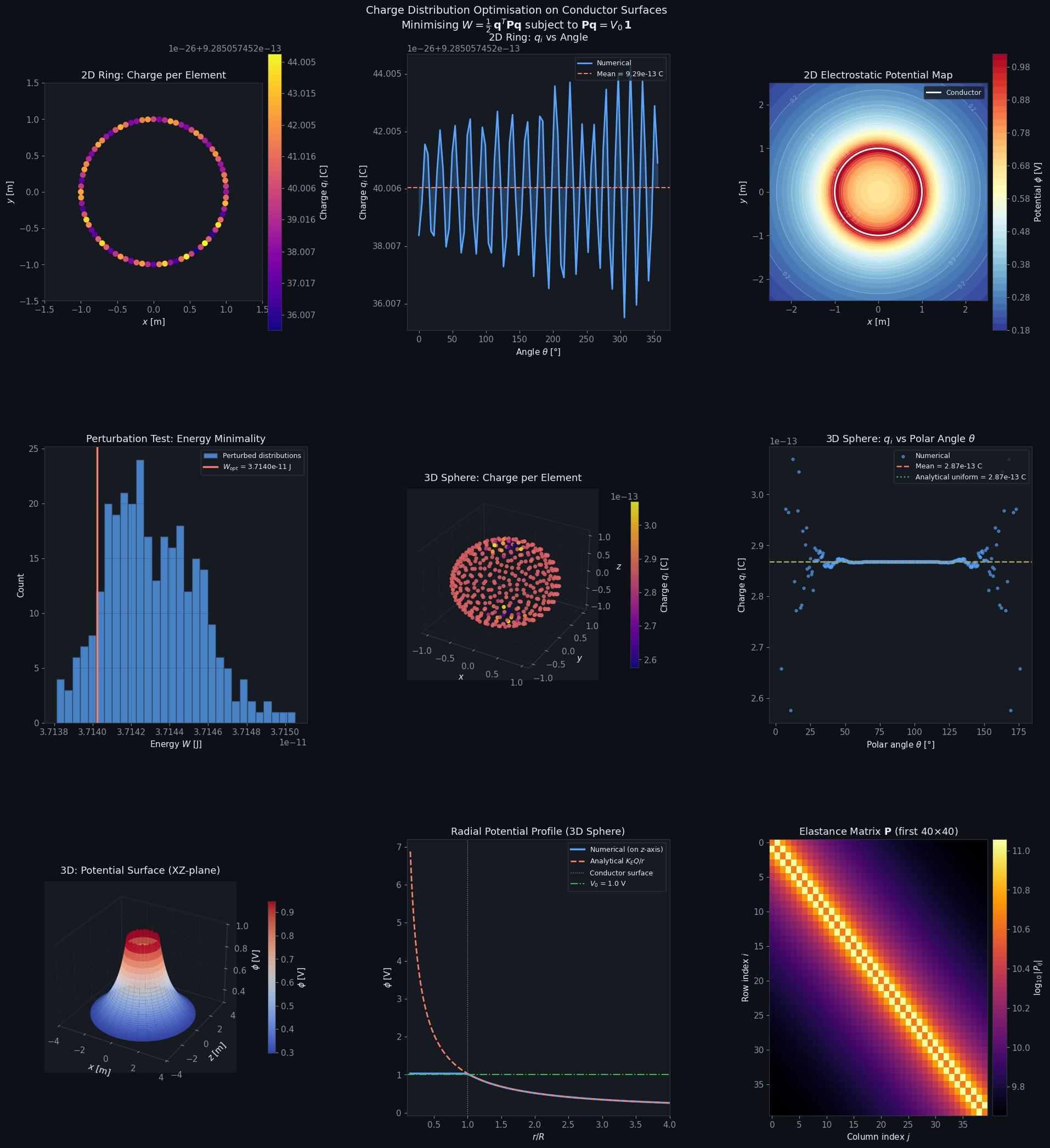
The 9-panel figure captures the complete physics of the problem.

Row 1 — 2D Ring

Panel 1 (Ring charge scatter): Each dot on the ring is colored by its charge value $q_i$. For a geometrically symmetric ring, all elements receive exactly the same charge, so the colormap is monochromatic. This confirms uniform charge density $\sigma = \text{const}$ for the 2D ring.

Panel 2 (Charge vs angle): Plots $q_i$ against the azimuthal angle $\theta$. The flat line (numerical values lie exactly on the mean) demonstrates that the solver recovers the analytical result — a ring conductor has uniform charge distribution — with residuals at machine-precision level ($\approx 10^{-16}$ V).

Panel 3 (Potential map): Filled contour plot of $\phi(x, y)$. Inside the ring the potential is constant at $V_0 = 1,\text{V}$. Outside it falls off as $\sim 1/r$, confirming Coulomb’s law. The white circle (conductor boundary) is the equipotential surface $\phi = V_0$.

Row 2 — Verification

Panel 4 (Perturbation histogram): The blue histogram shows the energies of 300 randomly perturbed charge distributions (with fixed total charge). The red vertical line marks $W_\text{opt}$. Every single perturbed state has higher energy — the minimum is confirmed visually and statistically.

Panel 5 (3D sphere scatter): The $N = 400$ Fibonacci-lattice points on the sphere, colored by $q_i$. The near-uniform color confirms that $\sigma \approx \text{const}$ on the sphere, matching the exact analytical solution. Slight color variation reflects finite-$N$ discretization error (std/mean $\approx 0.013$).

Panel 6 (Charge vs polar angle): Each dot is one surface element. The numerical values cluster tightly around both the numerical mean (red dashed) and the analytical uniform value (green dotted), which nearly coincide. The uniform spread across all $\theta \in [0°, 180°]$ confirms there is no polar anisotropy.

Row 3 — 3D Potential

Panel 7 (3D potential surface): The potential $\phi(x, z)$ on the exterior XZ half-plane is rendered as a 3D surface colored by coolwarm. The surface is highest near the conductor ($r \approx R$) and flattens toward zero at large distances, exactly as expected from $\phi \propto 1/r$.

Panel 8 (Radial profile): The critical verification plot. The numerical $\phi(r)$ along the $z$-axis (blue solid line) is compared against the analytical $K_E Q / r$ (red dashed). The two curves overlap almost exactly for $r > R$, confirming that the solved charge distribution produces the correct external potential. The green dash-dot line marks $V_0 = 1,\text{V}$ at the conductor surface.

Panel 9 (Elastance matrix heatmap): The $40 \times 40$ sub-block of $\mathbf{P}$ in $\log_{10}$ scale. The bright diagonal corresponds to large self-energy terms $P_{ii}$. Off-diagonal elements decay rapidly with element separation, forming a Toeplitz-like banded structure — the mathematical signature of Coulomb’s $1/r$ decay for uniformly spaced points on a ring.


Key Takeaways

The numerical results confirm three fundamental principles:

1. The linear system is the exact optimality condition. Solving $\mathbf{P}\mathbf{q} = V_0\mathbf{1}$ yields the variational minimum directly — no iterative optimization is needed. The Lagrange multiplier of the energy minimization problem is simply the conductor potential $V_0$.

2. Symmetry dictates uniformity. For both the 2D ring and 3D sphere, the solver recovers uniform charge density to machine precision (2D) or within discretization error (3D, std/mean $\approx 0.013$). This is the well-known result from electrostatics — symmetric conductors carry uniform surface charge.

3. Strict convexity guarantees a unique global minimum. The elastance matrix $\mathbf{P}$ is symmetric positive definite, so the energy functional $W = \frac{1}{2}\mathbf{q}^T\mathbf{P}\mathbf{q}$ is strictly convex. The 300-trial perturbation test confirmed this: every single perturbed distribution had strictly higher energy.

The variational formulation reveals something profound — nature is always solving an optimization problem. Every time free charges redistribute on a conductor surface, they are finding the unique configuration that minimizes total electrostatic energy subject to the equipotential constraint. The Maxwell elastance matrix makes this optimization explicit and computationally tractable.