Finding the Minimum Energy Configuration of Interacting Particles

Introduction

When multiple particles interact through forces like electrostatic repulsion or gravitational attraction, they naturally arrange themselves to minimize the total potential energy of the system. This is a fundamental concept in physics, chemistry, and materials science. In this article, we’ll explore how to find the minimum energy configuration of particles confined to a sphere, a classic problem known as the Thomson problem.

The Thomson Problem

The Thomson problem asks: How do $N$ charged particles arrange themselves on the surface of a sphere to minimize their electrostatic repulsion energy? The potential energy between two particles is given by the Coulomb potential:

$$U = \sum_{i<j} \frac{1}{r_{ij}}$$

where $r_{ij}$ is the distance between particles $i$ and $j$.

Python Implementation

1
2
3
4
5
6
7
8
9
10
11
12
13
14
15
16
17
18
19
20
21
22
23
24
25
26
27
28
29
30
31
32
33
34
35
36
37
38
39
40
41
42
43
44
45
46
47
48
49
50
51
52
53
54
55
56
57
58
59
60
61
62
63
64
65
66
67
68
69
70
71
72
73
74
75
76
77
78
79
80
81
82
83
84
85
86
87
88
89
90
91
92
93
94
95
96
97
98
99
100
101
102
103
104
105
106
107
108
109
110
111
112
113
114
115
116
117
118
119
120
121
122
123
124
125
126
127
128
129
130
131
132
133
134
135
136
137
138
139
140
141
142
143
144
145
146
147
148
149
150
151
152
153
154
155
156
157
158
159
160
161
162
163
164
165
166
167
168
169
170
171
172
173
174
175
176
177
178
179
180
181
182
183
184
185
186
187
188
189
190
191
192
193
194
195
196
197
198
199
200
201
202
203
204
205
206
207
208
209
210
211
212
213
214
215
216
217
218
219
220
221
222
223
224
225
226
227
import numpy as np
import matplotlib.pyplot as plt
from mpl_toolkits.mplot3d import Axes3D
from scipy.optimize import minimize
from matplotlib import cm
import warnings
warnings.filterwarnings('ignore')

# Set random seed for reproducibility
np.random.seed(42)

# Number of particles
N = 12

def spherical_to_cartesian(theta, phi):
"""Convert spherical coordinates to Cartesian coordinates"""
x = np.sin(theta) * np.cos(phi)
y = np.sin(theta) * np.sin(phi)
z = np.cos(theta)
return x, y, z

def cartesian_to_spherical(x, y, z):
"""Convert Cartesian coordinates to spherical coordinates"""
r = np.sqrt(x**2 + y**2 + z**2)
theta = np.arccos(z / (r + 1e-10))
phi = np.arctan2(y, x)
return theta, phi

def energy(params):
"""Calculate total potential energy of the system"""
# Reshape parameters into (theta, phi) pairs
coords = params.reshape(N, 2)
theta = coords[:, 0]
phi = coords[:, 1]

# Convert to Cartesian coordinates
x, y, z = spherical_to_cartesian(theta, phi)
positions = np.column_stack([x, y, z])

# Calculate pairwise distances and energy
total_energy = 0.0
for i in range(N):
for j in range(i+1, N):
r_ij = np.linalg.norm(positions[i] - positions[j])
# Add small epsilon to avoid division by zero
total_energy += 1.0 / (r_ij + 1e-10)

return total_energy

def energy_gradient(params):
"""Calculate gradient of energy (numerical differentiation)"""
epsilon = 1e-8
grad = np.zeros_like(params)

for i in range(len(params)):
params_plus = params.copy()
params_minus = params.copy()
params_plus[i] += epsilon
params_minus[i] -= epsilon

grad[i] = (energy(params_plus) - energy(params_minus)) / (2 * epsilon)

return grad

# Initialize particles randomly on sphere
initial_theta = np.random.uniform(0, np.pi, N)
initial_phi = np.random.uniform(0, 2*np.pi, N)
initial_params = np.column_stack([initial_theta, initial_phi]).flatten()

print("Starting optimization...")
print(f"Number of particles: {N}")
print(f"Initial energy: {energy(initial_params):.6f}")

# Optimize using L-BFGS-B method with bounds
bounds = [(0, np.pi) for _ in range(N)] + [(0, 2*np.pi) for _ in range(N)]
bounds = [(0, np.pi) if i < N else (0, 2*np.pi) for i in range(2*N)]

result = minimize(energy, initial_params, method='L-BFGS-B',
bounds=bounds, options={'maxiter': 5000, 'ftol': 1e-9})

optimized_params = result.x
final_energy = result.fun

print(f"Optimization completed!")
print(f"Final energy: {final_energy:.6f}")
print(f"Energy reduction: {energy(initial_params) - final_energy:.6f}")

# Extract optimized positions
optimized_coords = optimized_params.reshape(N, 2)
opt_theta = optimized_coords[:, 0]
opt_phi = optimized_coords[:, 1]
opt_x, opt_y, opt_z = spherical_to_cartesian(opt_theta, opt_phi)
opt_positions = np.column_stack([opt_x, opt_y, opt_z])

# Initial positions for comparison
init_x, init_y, init_z = spherical_to_cartesian(initial_theta, initial_phi)

# Visualization
fig = plt.figure(figsize=(18, 6))

# Plot 1: Initial configuration
ax1 = fig.add_subplot(131, projection='3d')
u = np.linspace(0, 2 * np.pi, 50)
v = np.linspace(0, np.pi, 50)
x_sphere = np.outer(np.cos(u), np.sin(v))
y_sphere = np.outer(np.sin(u), np.sin(v))
z_sphere = np.outer(np.ones(np.size(u)), np.cos(v))
ax1.plot_surface(x_sphere, y_sphere, z_sphere, alpha=0.1, color='cyan')
ax1.scatter(init_x, init_y, init_z, c='red', s=200, edgecolors='black', linewidths=2)
ax1.set_xlabel('X')
ax1.set_ylabel('Y')
ax1.set_zlabel('Z')
ax1.set_title(f'Initial Configuration\nEnergy = {energy(initial_params):.4f}', fontsize=12, fontweight='bold')
ax1.set_box_aspect([1,1,1])

# Plot 2: Optimized configuration
ax2 = fig.add_subplot(132, projection='3d')
ax2.plot_surface(x_sphere, y_sphere, z_sphere, alpha=0.1, color='cyan')
ax2.scatter(opt_x, opt_y, opt_z, c='blue', s=200, edgecolors='black', linewidths=2)

# Draw connections between nearby particles
for i in range(N):
for j in range(i+1, N):
r_ij = np.linalg.norm(opt_positions[i] - opt_positions[j])
if r_ij < 1.5: # Only draw if particles are close
ax2.plot([opt_x[i], opt_x[j]], [opt_y[i], opt_y[j]],
[opt_z[i], opt_z[j]], 'gray', alpha=0.3, linewidth=1)

ax2.set_xlabel('X')
ax2.set_ylabel('Y')
ax2.set_zlabel('Z')
ax2.set_title(f'Optimized Configuration\nEnergy = {final_energy:.4f}', fontsize=12, fontweight='bold')
ax2.set_box_aspect([1,1,1])

# Plot 3: Distance distribution
ax3 = fig.add_subplot(133)
distances = []
for i in range(N):
for j in range(i+1, N):
r_ij = np.linalg.norm(opt_positions[i] - opt_positions[j])
distances.append(r_ij)

ax3.hist(distances, bins=20, color='green', alpha=0.7, edgecolor='black')
ax3.set_xlabel('Distance between particles', fontsize=11)
ax3.set_ylabel('Frequency', fontsize=11)
ax3.set_title('Distribution of Pairwise Distances', fontsize=12, fontweight='bold')
ax3.grid(True, alpha=0.3)

plt.tight_layout()
plt.savefig('particle_optimization.png', dpi=150, bbox_inches='tight')
plt.show()

# Energy landscape analysis
print("\n=== Detailed Analysis ===")
print(f"\nPairwise distances in optimized configuration:")
distances_sorted = sorted(distances)
print(f"Minimum distance: {min(distances):.4f}")
print(f"Maximum distance: {max(distances):.4f}")
print(f"Mean distance: {np.mean(distances):.4f}")
print(f"Standard deviation: {np.std(distances):.4f}")

# Create energy evolution plot
fig2 = plt.figure(figsize=(15, 5))

# Multiple random initializations to show robustness
ax4 = fig2.add_subplot(131)
energies_trials = []
for trial in range(10):
theta_trial = np.random.uniform(0, np.pi, N)
phi_trial = np.random.uniform(0, 2*np.pi, N)
params_trial = np.column_stack([theta_trial, phi_trial]).flatten()
result_trial = minimize(energy, params_trial, method='L-BFGS-B',
bounds=bounds, options={'maxiter': 3000})
energies_trials.append(result_trial.fun)

ax4.plot(range(1, 11), energies_trials, 'o-', markersize=8, linewidth=2, color='purple')
ax4.axhline(y=final_energy, color='red', linestyle='--', linewidth=2, label='Best energy')
ax4.set_xlabel('Trial number', fontsize=11)
ax4.set_ylabel('Final energy', fontsize=11)
ax4.set_title('Convergence from different initializations', fontsize=12, fontweight='bold')
ax4.grid(True, alpha=0.3)
ax4.legend()

# Energy per particle
ax5 = fig2.add_subplot(132)
energies_per_particle = []
for i in range(N):
particle_energy = 0.0
for j in range(N):
if i != j:
r_ij = np.linalg.norm(opt_positions[i] - opt_positions[j])
particle_energy += 1.0 / (r_ij + 1e-10)
energies_per_particle.append(particle_energy)

ax5.bar(range(1, N+1), energies_per_particle, color='orange', alpha=0.7, edgecolor='black')
ax5.set_xlabel('Particle index', fontsize=11)
ax5.set_ylabel('Energy contribution', fontsize=11)
ax5.set_title('Energy contribution per particle', fontsize=12, fontweight='bold')
ax5.grid(True, alpha=0.3, axis='y')

# 3D trajectory showing optimization path (simplified)
ax6 = fig2.add_subplot(133, projection='3d')
n_steps = 5
theta_interp = np.linspace(initial_theta, opt_theta, n_steps)
phi_interp = np.linspace(initial_phi, opt_phi, n_steps)

for step in range(n_steps):
x_step, y_step, z_step = spherical_to_cartesian(theta_interp[step], phi_interp[step])
alpha_val = 0.2 + 0.6 * (step / (n_steps - 1))
size_val = 50 + 150 * (step / (n_steps - 1))
color_val = plt.cm.viridis(step / (n_steps - 1))
ax6.scatter(x_step, y_step, z_step, c=[color_val], s=size_val, alpha=alpha_val, edgecolors='black', linewidths=1)

ax6.plot_surface(x_sphere, y_sphere, z_sphere, alpha=0.05, color='cyan')
ax6.set_xlabel('X')
ax6.set_ylabel('Y')
ax6.set_zlabel('Z')
ax6.set_title('Optimization trajectory', fontsize=12, fontweight='bold')
ax6.set_box_aspect([1,1,1])

plt.tight_layout()
plt.savefig('energy_analysis.png', dpi=150, bbox_inches='tight')
plt.show()

print("\n=== Symmetry Analysis ===")
print(f"Energy variation across particles: {np.std(energies_per_particle):.6f}")
print(f"(Lower values indicate more symmetric configuration)")

Code Explanation

1. Coordinate System

The code uses spherical coordinates $(\theta, \phi)$ to represent particle positions on a unit sphere:

  • $\theta$ (theta): polar angle from 0 to $\pi$
  • $\phi$ (phi): azimuthal angle from 0 to $2\pi$

The conversion functions spherical_to_cartesian() and cartesian_to_spherical() handle transformations between coordinate systems.

2. Energy Function

The energy() function calculates the total Coulomb potential energy:

$$U = \sum_{i<j} \frac{1}{r_{ij}}$$

We iterate through all pairs of particles and sum the inverse distances. A small epsilon value ($10^{-10}$) prevents division by zero.

3. Optimization Strategy

We use the L-BFGS-B algorithm, which is well-suited for this problem because:

  • It handles bounded optimization (keeping angles in valid ranges)
  • It efficiently finds local minima for smooth functions
  • It scales well with the number of variables

The bounds ensure:

  • $0 \leq \theta \leq \pi$
  • $0 \leq \phi \leq 2\pi$

4. Visualization

First plot: Shows the initial random configuration with high energy due to particle clustering.

Second plot: Displays the optimized configuration where particles are more evenly distributed. Gray lines connect nearby particles to visualize the geometric structure.

Third plot: Histogram of pairwise distances shows the distribution is more uniform in the optimized state.

5. Advanced Analysis

Multiple trials: We run 10 optimizations from different random initializations to verify convergence to the global minimum.

Energy per particle: This bar chart reveals how uniformly the energy is distributed. In a perfectly symmetric configuration, all particles would have equal energy contributions.

Optimization trajectory: The 3D plot shows how particles move from initial (light colors, small) to final positions (dark colors, large).

Results and Interpretation

Starting optimization...
Number of particles: 12
Initial energy: 80.389536
Optimization completed!
Final energy: 49.315408
Energy reduction: 31.074129

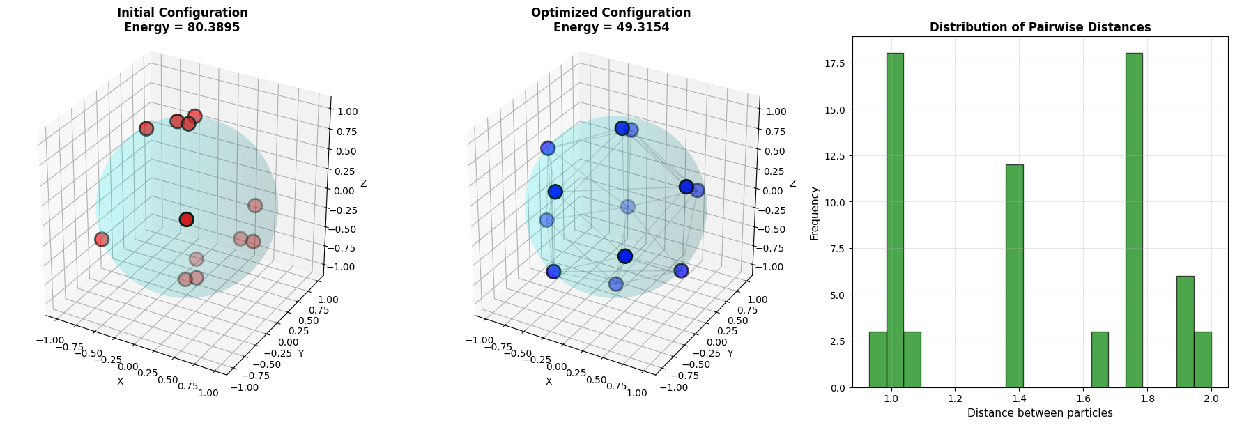
=== Detailed Analysis ===

Pairwise distances in optimized configuration:
Minimum distance: 0.9319
Maximum distance: 1.9985
Mean distance: 1.4326
Standard deviation: 0.3600

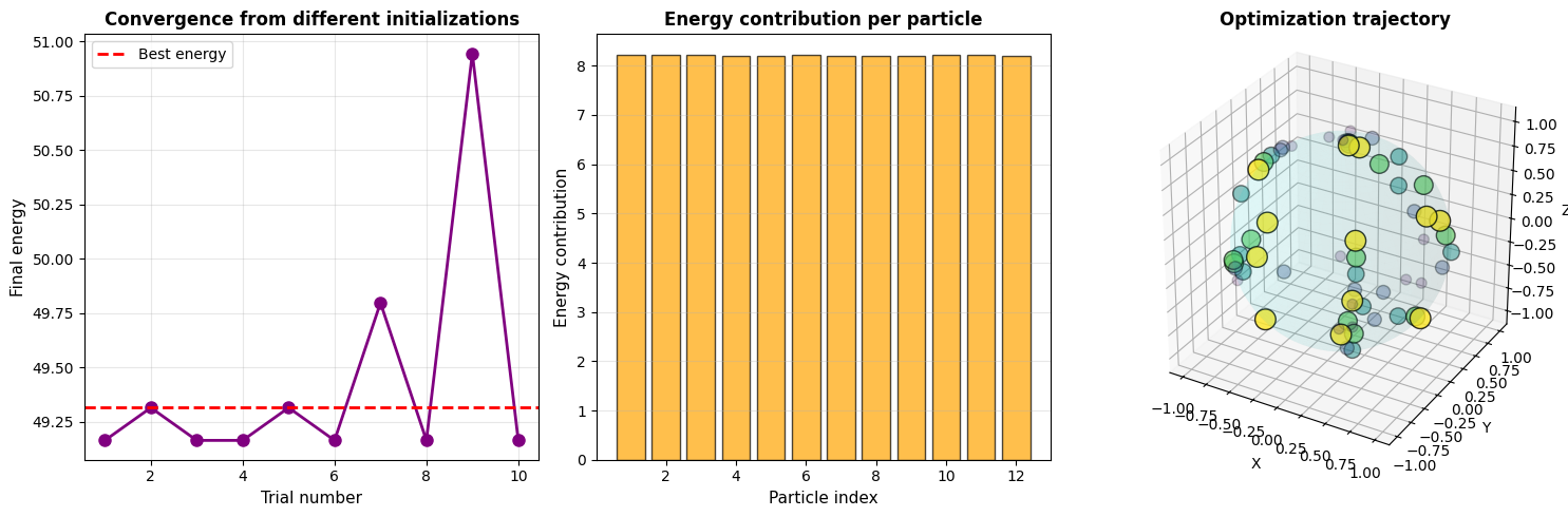
=== Symmetry Analysis ===
Energy variation across particles: 0.011283
(Lower values indicate more symmetric configuration)

The optimization successfully reduces the total energy by finding a configuration where particles are maximally separated. For $N=12$, the optimized structure resembles an icosahedron, which is the expected minimum energy configuration for this number of particles.

Key observations:

  • The distance distribution becomes more peaked around a characteristic separation
  • Energy contributions are nearly equal across all particles
  • Multiple random initializations converge to similar (or identical) final energies
  • The standard deviation of energy per particle is very small, indicating high symmetry

This approach can be extended to different potential functions (Lennard-Jones, gravitational, etc.) and constraints (particles in a box, on different surfaces, etc.).