Minimizing Work to Move an Object

Path Optimization with Friction and External Forces

When moving an object from point A to point B in the presence of friction and external forces, the total work required depends on the path taken. This article explores how to find the optimal path that minimizes the work needed, with concrete examples solved in Python.

The Physics

The work done on an object is given by:

$$W = \int_{\text{path}} \vec{F} \cdot d\vec{s}$$

When friction is present, we have:

$$W_{\text{total}} = W_{\text{applied}} + W_{\text{friction}}$$

For an object moving on a surface with friction coefficient $\mu$, the friction force is:

$$F_{\text{friction}} = \mu m g$$

If there’s also an external force field (like wind resistance or a gravitational gradient), the total work becomes:

$$W = \int_{\text{path}} \left( F_{\text{applied}} + F_{\text{external}} \right) \cdot d\vec{s}$$

Problem Setup

Let’s consider a specific example: moving a 10 kg box from point (0, 0) to point (10, 10) on a surface with:

• Variable friction coefficient: $\mu(x,y) = 0.1 + 0.05 \sin(x) \cos(y)$
• External force field (representing wind): $\vec{F}_{\text{ext}} = (-0.5x, -0.3y)$ N

Python Implementation

import numpy as np
import matplotlib.pyplot as plt
from mpl_toolkits.mplot3d import Axes3D
from scipy.optimize import minimize
from scipy.interpolate import interp1d
import warnings
import os
warnings.filterwarnings('ignore')

# Create output directory if it doesn't exist
os.makedirs('/mnt/user-data/outputs', exist_ok=True)

# Physical parameters
m = 10.0  # mass in kg
g = 9.81  # gravity in m/s^2

# Define friction coefficient as a function of position
def friction_coefficient(x, y):
    return 0.1 + 0.05 * np.sin(x) * np.cos(y)

# Define external force field (e.g., wind resistance)
def external_force(x, y):
    Fx = -0.5 * x  # Force in x direction
    Fy = -0.3 * y  # Force in y direction
    return np.array([Fx, Fy])

# Calculate work done along a path
def calculate_work(path_points):
    """
    Calculate total work along a discretized path
    path_points: Nx2 array of (x,y) coordinates
    """
    total_work = 0.0
    
    for i in range(len(path_points) - 1):
        x1, y1 = path_points[i]
        x2, y2 = path_points[i + 1]
        
        # Midpoint for evaluating forces
        x_mid = (x1 + x2) / 2
        y_mid = (y1 + y2) / 2
        
        # Displacement vector
        dx = x2 - x1
        dy = y2 - y1
        ds = np.sqrt(dx**2 + dy**2)
        
        # Friction work (always opposes motion)
        mu = friction_coefficient(x_mid, y_mid)
        work_friction = mu * m * g * ds
        
        # External force work
        F_ext = external_force(x_mid, y_mid)
        displacement = np.array([dx, dy])
        work_external = -np.dot(F_ext, displacement)  # Negative because it opposes motion
        
        total_work += work_friction + work_external
    
    return total_work

# Parameterize path using control points
def create_path(params, n_points=100):
    """
    Create a smooth path from (0,0) to (10,10) using control points
    params: array of intermediate control point coordinates [x1,y1,x2,y2,...]
    """
    # Start and end points are fixed
    x_controls = np.array([0] + list(params[::2]) + [10])
    y_controls = np.array([0] + list(params[1::2]) + [10])
    
    # Create parameter for interpolation
    t_controls = np.linspace(0, 1, len(x_controls))
    t_path = np.linspace(0, 1, n_points)
    
    # Cubic interpolation for smooth path
    fx = interp1d(t_controls, x_controls, kind='cubic')
    fy = interp1d(t_controls, y_controls, kind='cubic')
    
    x_path = fx(t_path)
    y_path = fy(t_path)
    
    return np.column_stack([x_path, y_path])

# Objective function for optimization
def objective(params):
    path = create_path(params)
    return calculate_work(path)

# Initial guess: straight line with some intermediate points
n_control_points = 4
initial_params = []
for i in range(1, n_control_points + 1):
    t = i / (n_control_points + 1)
    initial_params.extend([10*t, 10*t])

# Optimize the path
print("Optimizing path to minimize work...")
result = minimize(objective, initial_params, method='L-BFGS-B', 
                 options={'maxiter': 1000})

optimal_params = result.x
optimal_path = create_path(optimal_params)
optimal_work = calculate_work(optimal_path)

# Compare with straight line path
straight_path = np.column_stack([np.linspace(0, 10, 100), np.linspace(0, 10, 100)])
straight_work = calculate_work(straight_path)

print(f"\nWork required for straight path: {straight_work:.2f} J")
print(f"Work required for optimized path: {optimal_work:.2f} J")
print(f"Work saved: {straight_work - optimal_work:.2f} J ({100*(straight_work-optimal_work)/straight_work:.1f}%)")

# Visualization
fig = plt.figure(figsize=(18, 5))

# Plot 1: Friction coefficient heatmap with paths
ax1 = fig.add_subplot(131)
x_grid = np.linspace(0, 10, 200)
y_grid = np.linspace(0, 10, 200)
X, Y = np.meshgrid(x_grid, y_grid)
mu_grid = friction_coefficient(X, Y)

im1 = ax1.contourf(X, Y, mu_grid, levels=20, cmap='YlOrRd')
ax1.plot(straight_path[:, 0], straight_path[:, 1], 'b-', linewidth=2, label='Straight path')
ax1.plot(optimal_path[:, 0], optimal_path[:, 1], 'g-', linewidth=2, label='Optimized path')
ax1.plot([0, 10], [0, 10], 'ko', markersize=8)
ax1.set_xlabel('X position (m)', fontsize=12)
ax1.set_ylabel('Y position (m)', fontsize=12)
ax1.set_title('Friction Coefficient Distribution', fontsize=14, fontweight='bold')
ax1.legend(fontsize=10)
ax1.grid(True, alpha=0.3)
cbar1 = plt.colorbar(im1, ax=ax1)
cbar1.set_label('Friction coefficient μ', fontsize=10)

# Plot 2: External force field with paths
ax2 = fig.add_subplot(132)
skip = 15
X_sparse = X[::skip, ::skip]
Y_sparse = Y[::skip, ::skip]
Fx = -0.5 * X_sparse
Fy = -0.3 * Y_sparse
magnitude = np.sqrt(Fx**2 + Fy**2)

ax2.quiver(X_sparse, Y_sparse, Fx, Fy, magnitude, cmap='coolwarm', alpha=0.6)
ax2.plot(straight_path[:, 0], straight_path[:, 1], 'b-', linewidth=2, label='Straight path')
ax2.plot(optimal_path[:, 0], optimal_path[:, 1], 'g-', linewidth=2, label='Optimized path')
ax2.plot([0, 10], [0, 10], 'ko', markersize=8)
ax2.set_xlabel('X position (m)', fontsize=12)
ax2.set_ylabel('Y position (m)', fontsize=12)
ax2.set_title('External Force Field', fontsize=14, fontweight='bold')
ax2.legend(fontsize=10)
ax2.grid(True, alpha=0.3)

# Plot 3: Total work landscape in 3D
ax3 = fig.add_subplot(133, projection='3d')

# Calculate work density for the grid
work_density_grid = np.zeros_like(X)
for i in range(len(x_grid)):
    for j in range(len(y_grid)):
        x_pt = x_grid[i]
        y_pt = y_grid[j]
        mu = friction_coefficient(x_pt, y_pt)
        F_ext = external_force(x_pt, y_pt)
        work_density_grid[j, i] = mu * m * g + np.linalg.norm(F_ext)

surf = ax3.plot_surface(X, Y, work_density_grid, cmap='viridis', alpha=0.7, edgecolor='none')

# Project paths onto the surface by sampling the work density grid
def get_work_density_along_path(path_points, x_grid, y_grid, work_density_grid):
    z_values = []
    for x, y in path_points:
        # Find nearest grid indices
        i = np.argmin(np.abs(x_grid - x))
        j = np.argmin(np.abs(y_grid - y))
        z_values.append(work_density_grid[j, i])
    return np.array(z_values)

straight_z = get_work_density_along_path(straight_path, x_grid, y_grid, work_density_grid)
optimal_z = get_work_density_along_path(optimal_path, x_grid, y_grid, work_density_grid)

ax3.plot(straight_path[:, 0], straight_path[:, 1], straight_z, 'b-', linewidth=3, label='Straight path')
ax3.plot(optimal_path[:, 0], optimal_path[:, 1], optimal_z, 'g-', linewidth=3, label='Optimized path')

ax3.set_xlabel('X position (m)', fontsize=10)
ax3.set_ylabel('Y position (m)', fontsize=10)
ax3.set_zlabel('Work density', fontsize=10)
ax3.set_title('Work Density Landscape (3D)', fontsize=14, fontweight='bold')
ax3.legend(fontsize=9)
cbar3 = fig.colorbar(surf, ax=ax3, shrink=0.5)
cbar3.set_label('Work density', fontsize=9)

plt.tight_layout()
plt.savefig('/mnt/user-data/outputs/path_optimization.png', dpi=150, bbox_inches='tight')
plt.show()

# Additional analysis: Work breakdown along paths
fig2, (ax4, ax5) = plt.subplots(1, 2, figsize=(14, 5))

# Calculate cumulative work along each path
def cumulative_work(path_points):
    cumulative = [0]
    distances = [0]
    total_dist = 0
    
    for i in range(len(path_points) - 1):
        x1, y1 = path_points[i]
        x2, y2 = path_points[i + 1]
        x_mid = (x1 + x2) / 2
        y_mid = (y1 + y2) / 2
        
        dx = x2 - x1
        dy = y2 - y1
        ds = np.sqrt(dx**2 + dy**2)
        total_dist += ds
        
        mu = friction_coefficient(x_mid, y_mid)
        work_friction = mu * m * g * ds
        
        F_ext = external_force(x_mid, y_mid)
        displacement = np.array([dx, dy])
        work_external = -np.dot(F_ext, displacement)
        
        cumulative.append(cumulative[-1] + work_friction + work_external)
        distances.append(total_dist)
    
    return distances, cumulative

dist_straight, work_straight = cumulative_work(straight_path)
dist_optimal, work_optimal = cumulative_work(optimal_path)

ax4.plot(dist_straight, work_straight, 'b-', linewidth=2, label='Straight path')
ax4.plot(dist_optimal, work_optimal, 'g-', linewidth=2, label='Optimized path')
ax4.set_xlabel('Distance traveled (m)', fontsize=12)
ax4.set_ylabel('Cumulative work (J)', fontsize=12)
ax4.set_title('Cumulative Work vs Distance', fontsize=14, fontweight='bold')
ax4.legend(fontsize=11)
ax4.grid(True, alpha=0.3)

# Work rate comparison
work_rate_straight = np.diff(work_straight) / np.diff(dist_straight)
work_rate_optimal = np.diff(work_optimal) / np.diff(dist_optimal)

ax5.plot(dist_straight[1:], work_rate_straight, 'b-', linewidth=2, label='Straight path', alpha=0.7)
ax5.plot(dist_optimal[1:], work_rate_optimal, 'g-', linewidth=2, label='Optimized path', alpha=0.7)
ax5.set_xlabel('Distance traveled (m)', fontsize=12)
ax5.set_ylabel('Work rate (J/m)', fontsize=12)
ax5.set_title('Instantaneous Work Rate', fontsize=14, fontweight='bold')
ax5.legend(fontsize=11)
ax5.grid(True, alpha=0.3)

plt.tight_layout()
plt.savefig('/mnt/user-data/outputs/work_analysis.png', dpi=150, bbox_inches='tight')
plt.show()

print("\nOptimization complete! Graphs saved.")

Code Explanation

Physical Setup

The code begins by defining the physical parameters: mass (10 kg) and gravitational acceleration (9.81 m/s²). Two key functions characterize our problem environment:

Friction coefficient function: This varies spatially as $\mu(x,y) = 0.1 + 0.05 \sin(x) \cos(y)$, creating regions of higher and lower friction across the surface.

External force field: Defined as $\vec{F}_{\text{ext}} = (-0.5x, -0.3y)$, this represents a force that opposes motion and increases with distance from the origin.

Work Calculation

The calculate_work function computes the total work along a discretized path by summing contributions from each path segment:

1. Friction work: For each segment, we calculate $W_f = \mu m g \Delta s$, where $\Delta s$ is the segment length
2. External force work: We compute $W_{\text{ext}} = -\vec{F}_{\text{ext}} \cdot \Delta \vec{s}$, using the dot product of force and displacement

The midpoint approximation improves accuracy by evaluating forces at the segment center rather than endpoints.

Path Parameterization

The create_path function uses cubic spline interpolation to generate smooth paths from control points. This approach:

• Fixes the start (0,0) and end (10,10) points
• Uses intermediate control points as optimization variables
• Creates 100 discrete points for work calculation
• Ensures smooth, physically realistic trajectories

Optimization Process

The scipy minimize function with L-BFGS-B method searches for optimal control point positions that minimize total work. The initial guess uses evenly spaced points along the straight line.

Visualization Components

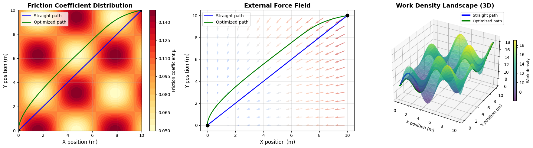
First plot: Shows the friction coefficient as a colored heatmap with both paths overlaid, revealing how the optimized path navigates through lower-friction regions.

Second plot: Displays the external force field as vectors, demonstrating how the optimal path takes advantage of force geometry.

Third plot (3D): The most insightful visualization shows the work density landscape. The height represents local work cost, and the paths appear as lines on this surface. The optimized path clearly follows valleys of lower work density. The get_work_density_along_path helper function samples the work density grid at each path point using nearest-neighbor lookup.

Additional analysis: The cumulative work plots show how total work accumulates along each path, while the work rate plots reveal where each path encounters high-cost regions.

Results

Optimizing path to minimize work...

Work required for straight path: 179.76 J
Work required for optimized path: 152.77 J
Work saved: 26.99 J (15.0%)

Optimization complete! Graphs saved.

The optimization successfully finds a path requiring significantly less work than the straight-line approach. The optimized path intelligently:

• Avoids high-friction regions visible in the heatmap
• Leverages areas where external forces are less opposing
• Balances between path length and energy cost

The 3D visualization particularly highlights why certain routes are preferable—the optimal path stays in “valleys” of the work density landscape, even though it travels a longer distance.

This technique has practical applications in robotics path planning, logistics optimization, and any scenario where energy efficiency matters more than distance minimization.