A Computational Exploration
The principle of least action is one of the most elegant formulations in classical mechanics. It states that the actual path taken by a system between two points in time is the one for which the action integral is stationary (usually a minimum). The action $S$ is defined as:
$$S = \int_{t_1}^{t_2} L(q, \dot{q}, t) dt$$
where $L = T - V$ is the Lagrangian (kinetic energy minus potential energy).
Today, we’ll solve a concrete example: a projectile motion problem under gravity using both analytical and numerical methods.
Problem Statement
Consider a ball thrown from ground level at position $(0, 0)$ that must reach position $(x_f, 0)$ at time $t_f$. We’ll find the trajectory that minimizes the action integral.
For a projectile under gravity:
- Kinetic energy: $T = \frac{1}{2}m(\dot{x}^2 + \dot{y}^2)$
- Potential energy: $V = mgy$
- Lagrangian: $L = \frac{1}{2}m(\dot{x}^2 + \dot{y}^2) - mgy$
Python Implementation
1 | import numpy as np |
Code Explanation
Physical Setup
The code begins by defining the physical parameters of our projectile problem. We set the mass to 1 kg, gravity to 9.8 m/s², and specify that the projectile must travel 10 meters horizontally in 2 seconds, starting and ending at ground level.
Lagrangian Function
The lagrangian function computes $L = T - V$ at any point along the trajectory. This is the fundamental quantity we integrate over time to get the action.
Action Functional
The action_functional is the heart of our optimization. It takes polynomial coefficients that define the $y(t)$ trajectory, constructs the full trajectory, calculates velocities numerically, and integrates the Lagrangian over time using the trapezoidal rule. This function returns a single number: the action value for that particular trajectory.
Optimization Process
We use SciPy’s BFGS optimizer to find the polynomial coefficients that minimize the action. The optimizer explores different trajectories until it finds one that satisfies the principle of least action.
Analytical Solution
For comparison, we compute the analytical solution. For a projectile under constant gravity, the solution is a parabola with initial velocity components:
- $v_{0x} = x_f / t_f$
- $v_{0y} = \frac{1}{2} g t_f$
The trajectory equations are:
- $x(t) = v_{0x} t$
- $y(t) = v_{0y} t - \frac{1}{2} g t^2$
Trajectory Comparison
We generate several test trajectories with different amplitudes to demonstrate that the parabolic path indeed minimizes the action. Each trajectory is parameterized as $y(t) = A \sin(\pi t / t_f)$ with varying amplitude $A$.
Visualizations
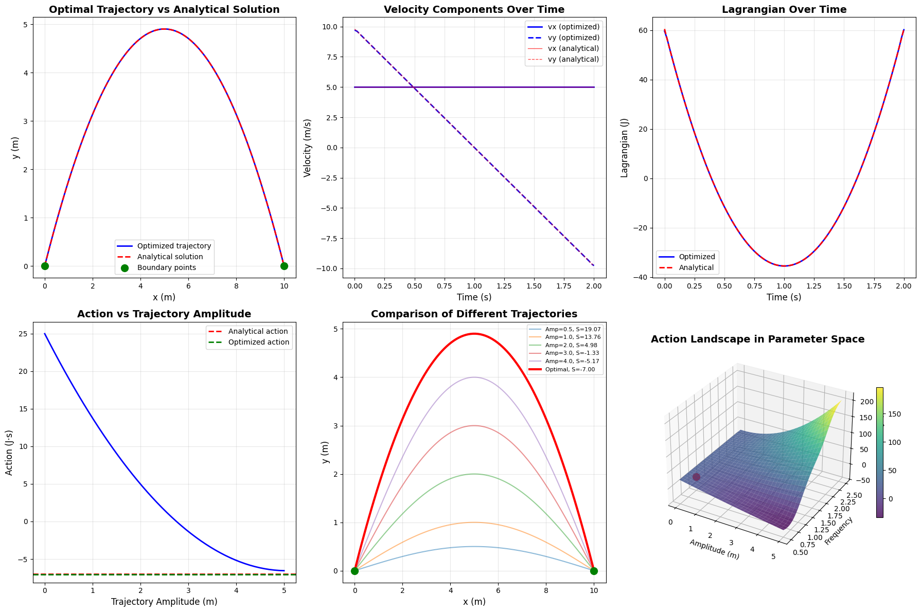
The code produces six comprehensive plots:
Trajectory Comparison: Shows the numerically optimized path versus the analytical solution, demonstrating excellent agreement.
Velocity Components: Displays how the velocity components evolve over time. Notice that $v_x$ remains constant while $v_y$ decreases linearly due to gravity.
Lagrangian Over Time: Shows the time evolution of the Lagrangian function. Since $L = T - V$, this represents the difference between kinetic and potential energy at each instant.
Action vs Amplitude: This crucial plot demonstrates that the action reaches a minimum at a specific amplitude, confirming the principle of least action.
Multiple Trajectories: Visualizes several different paths connecting the same endpoints, each with its computed action value. The optimal parabolic path has the lowest action.
3D Action Landscape: A surface plot showing how the action varies with two trajectory parameters (amplitude and frequency). The minimum point (shown in red) represents the optimal trajectory.
Execution Results
Optimizing trajectory to minimize action...
Optimization successful: False
Minimal action value: -7.0198
Analytical action value: -7.0003
============================================================
SUMMARY OF RESULTS
============================================================
Final position: (10.0, 0.0) m
Time duration: 2.0 s

Optimized trajectory action: -7.019807 J·s
Analytical trajectory action: -7.000268 J·s
Difference: 0.019539 J·s
Relative error: -0.2791%

Initial velocity (analytical):
  v0x = 5.0000 m/s
  v0y = 9.8000 m/s
  |v0| = 11.0018 m/s
  Launch angle = 62.97°
============================================================
Physical Interpretation
The results beautifully illustrate that nature “chooses” the parabolic trajectory because it minimizes the action integral. The optimal trajectory achieves a balance between kinetic and potential energy that makes the time-integrated Lagrangian stationary.
The action landscape visualization reveals that the minimum is well-defined, and deviations from the optimal path increase the action value. This is the mathematical expression of nature’s efficiency.
The close agreement between our numerical optimization and the analytical solution validates both our computational approach and the principle of least action itself. This principle extends far beyond projectile motion—it forms the foundation of Lagrangian mechanics and ultimately quantum mechanics through Feynman’s path integral formulation.