The Brachistochrone Problem

Finding the Fastest Path Under Gravity

The brachistochrone problem is one of the most famous problems in the calculus of variations. It asks: what is the shape of the curve down which a bead sliding from rest and accelerated by gravity will slip (without friction) from one point to another in the least time?

Surprisingly, the answer is not a straight line, but a cycloid - the curve traced by a point on the rim of a circle as it rolls along a straight line.

Mathematical Formulation

Given two points $A(0, 0)$ and $B(x_1, y_1)$ where $y_1 < 0$ (B is below A), we want to find the curve $y(x)$ that minimizes the travel time.

The time functional is:

$$T = \int_0^{x_1} \frac{\sqrt{1 + (y’)^2}}{\sqrt{2gy}} dx$$

Using the Euler-Lagrange equation, the solution is a cycloid parametrized as:

$$x(\theta) = r(\theta - \sin\theta)$$
$$y(\theta) = -r(1 - \cos\theta)$$

where $r$ is determined by the boundary condition at point B.

Specific Example Problem

Let’s solve a concrete example: A bead slides from point A(0, 0) to point B(2, -1) under gravity ($g = 9.8 , \text{m/s}^2$). We’ll compare three paths:

  1. Brachistochrone (Cycloid) - the optimal curve
  2. Straight line - the shortest distance
  3. Parabolic path - a smooth alternative

Python Implementation

1
2
3
4
5
6
7
8
9
10
11
12
13
14
15
16
17
18
19
20
21
22
23
24
25
26
27
28
29
30
31
32
33
34
35
36
37
38
39
40
41
42
43
44
45
46
47
48
49
50
51
52
53
54
55
56
57
58
59
60
61
62
63
64
65
66
67
68
69
70
71
72
73
74
75
76
77
78
79
80
81
82
83
84
85
86
87
88
89
90
91
92
93
94
95
96
97
98
99
100
101
102
103
104
105
106
107
108
109
110
111
112
113
114
115
116
117
118
119
120
121
122
123
124
125
126
127
128
129
130
131
132
133
134
135
136
137
138
139
140
141
142
143
144
145
146
147
148
149
150
151
152
153
154
155
156
157
158
159
160
161
162
163
164
165
166
167
168
169
170
171
172
173
174
175
176
177
178
179
180
181
182
183
184
185
186
187
188
189
190
191
192
193
194
195
196
197
198
199
200
201
202
203
204
205
206
207
208
209
210
211
212
213
214
215
216
217
218
219
220
221
222
223
224
225
226
227
228
229
230
231
232
233
234
235
import numpy as np
import matplotlib.pyplot as plt
from scipy.integrate import odeint, quad
from scipy.optimize import fsolve
from mpl_toolkits.mplot3d import Axes3D

# Physical constants
g = 9.8 # gravity (m/s^2)

# Boundary conditions
x0, y0 = 0.0, 0.0 # Start point A
x1, y1 = 2.0, -1.0 # End point B

# 1. Brachistochrone (Cycloid) solution
def find_cycloid_parameter(x_target, y_target):
"""Find the parameter r for cycloid passing through (x_target, y_target)"""
def equations(params):
r, theta_end = params
x = r * (theta_end - np.sin(theta_end))
y = -r * (1 - np.cos(theta_end))
return [x - x_target, y - y_target]

# Initial guess
r_guess = np.sqrt(x_target**2 + y_target**2) / 2
theta_guess = np.pi
solution = fsolve(equations, [r_guess, theta_guess])
return solution[0], solution[1]

# Find cycloid parameters
r_cycloid, theta_max = find_cycloid_parameter(x1, y1)

# Generate cycloid curve
theta_array = np.linspace(0, theta_max, 500)
x_cycloid = r_cycloid * (theta_array - np.sin(theta_array))
y_cycloid = -r_cycloid * (1 - np.cos(theta_array))

# 2. Straight line path
x_line = np.linspace(x0, x1, 500)
y_line = y0 + (y1 - y0) / (x1 - x0) * (x_line - x0)

# 3. Parabolic path
x_parabola = np.linspace(x0, x1, 500)
# Parabola passing through (0,0) and (x1,y1) with vertex control
a_para = y1 / (x1**2)
y_parabola = a_para * x_parabola**2

# Function to calculate travel time along a curve
def calculate_travel_time(x_path, y_path):
"""Calculate time to travel along a path under gravity"""
time = 0.0
for i in range(1, len(x_path)):
dx = x_path[i] - x_path[i-1]
dy = y_path[i] - y_path[i-1]
y_avg = (y_path[i] + y_path[i-1]) / 2

if y_avg >= 0: # No motion if above starting point
continue

ds = np.sqrt(dx**2 + dy**2)
v_avg = np.sqrt(2 * g * abs(y_avg))

if v_avg > 0:
time += ds / v_avg

return time

# Calculate times for each path
time_cycloid = calculate_travel_time(x_cycloid, y_cycloid)
time_line = calculate_travel_time(x_line, y_line)
time_parabola = calculate_travel_time(x_parabola, y_parabola)

# Calculate velocities along each path
def calculate_velocity_profile(x_path, y_path):
"""Calculate velocity at each point along the path"""
velocities = np.zeros(len(y_path))
for i in range(len(y_path)):
if y_path[i] < 0:
velocities[i] = np.sqrt(2 * g * abs(y_path[i]))
return velocities

v_cycloid = calculate_velocity_profile(x_cycloid, y_cycloid)
v_line = calculate_velocity_profile(x_line, y_line)
v_parabola = calculate_velocity_profile(x_parabola, y_parabola)

# Visualization
fig = plt.figure(figsize=(18, 12))

# Plot 1: Path comparison
ax1 = plt.subplot(2, 3, 1)
ax1.plot(x_cycloid, y_cycloid, 'b-', linewidth=2.5, label=f'Brachistochrone (t={time_cycloid:.4f}s)')
ax1.plot(x_line, y_line, 'r--', linewidth=2, label=f'Straight line (t={time_line:.4f}s)')
ax1.plot(x_parabola, y_parabola, 'g:', linewidth=2, label=f'Parabola (t={time_parabola:.4f}s)')
ax1.plot([x0, x1], [y0, y1], 'ko', markersize=10)
ax1.text(x0-0.1, y0+0.1, 'A', fontsize=14, fontweight='bold')
ax1.text(x1+0.1, y1, 'B', fontsize=14, fontweight='bold')
ax1.set_xlabel('x (m)', fontsize=12)
ax1.set_ylabel('y (m)', fontsize=12)
ax1.set_title('Path Comparison', fontsize=14, fontweight='bold')
ax1.legend(fontsize=10)
ax1.grid(True, alpha=0.3)
ax1.axis('equal')

# Plot 2: Velocity profiles
ax2 = plt.subplot(2, 3, 2)
ax2.plot(x_cycloid, v_cycloid, 'b-', linewidth=2.5, label='Brachistochrone')
ax2.plot(x_line, v_line, 'r--', linewidth=2, label='Straight line')
ax2.plot(x_parabola, v_parabola, 'g:', linewidth=2, label='Parabola')
ax2.set_xlabel('x (m)', fontsize=12)
ax2.set_ylabel('Velocity (m/s)', fontsize=12)
ax2.set_title('Velocity Along Path', fontsize=14, fontweight='bold')
ax2.legend(fontsize=10)
ax2.grid(True, alpha=0.3)

# Plot 3: Time comparison bar chart
ax3 = plt.subplot(2, 3, 3)
paths = ['Brachistochrone', 'Straight Line', 'Parabola']
times = [time_cycloid, time_line, time_parabola]
colors = ['blue', 'red', 'green']
bars = ax3.bar(paths, times, color=colors, alpha=0.7, edgecolor='black', linewidth=2)
ax3.set_ylabel('Travel Time (s)', fontsize=12)
ax3.set_title('Time Comparison', fontsize=14, fontweight='bold')
ax3.grid(True, alpha=0.3, axis='y')
for i, (bar, time) in enumerate(zip(bars, times)):
height = bar.get_height()
ax3.text(bar.get_x() + bar.get_width()/2., height,
f'{time:.4f}s\n({(time/time_cycloid-1)*100:+.1f}%)',
ha='center', va='bottom', fontsize=10, fontweight='bold')

# Plot 4: Cycloid generation (rolling circle)
ax4 = plt.subplot(2, 3, 4)
n_circles = 6
theta_samples = np.linspace(0, theta_max, n_circles)
for theta in theta_samples:
# Circle position
cx = r_cycloid * theta
cy = -r_cycloid
circle = plt.Circle((cx, cy), r_cycloid, fill=False, color='gray',
linestyle='--', alpha=0.5, linewidth=1)
ax4.add_patch(circle)
# Point on circle
px = r_cycloid * (theta - np.sin(theta))
py = -r_cycloid * (1 - np.cos(theta))
ax4.plot(px, py, 'ro', markersize=6, alpha=0.7)

ax4.plot(x_cycloid, y_cycloid, 'b-', linewidth=2.5, label='Cycloid curve')
ax4.set_xlabel('x (m)', fontsize=12)
ax4.set_ylabel('y (m)', fontsize=12)
ax4.set_title('Cycloid Generation (Rolling Circle)', fontsize=14, fontweight='bold')
ax4.legend(fontsize=10)
ax4.grid(True, alpha=0.3)
ax4.axis('equal')

# Plot 5: Path length comparison
def calculate_path_length(x_path, y_path):
length = 0.0
for i in range(1, len(x_path)):
dx = x_path[i] - x_path[i-1]
dy = y_path[i] - y_path[i-1]
length += np.sqrt(dx**2 + dy**2)
return length

length_cycloid = calculate_path_length(x_cycloid, y_cycloid)
length_line = calculate_path_length(x_line, y_line)
length_parabola = calculate_path_length(x_parabola, y_parabola)

ax5 = plt.subplot(2, 3, 5)
lengths = [length_cycloid, length_line, length_parabola]
bars2 = ax5.bar(paths, lengths, color=colors, alpha=0.7, edgecolor='black', linewidth=2)
ax5.set_ylabel('Path Length (m)', fontsize=12)
ax5.set_title('Path Length Comparison', fontsize=14, fontweight='bold')
ax5.grid(True, alpha=0.3, axis='y')
for bar, length in zip(bars2, lengths):
height = bar.get_height()
ax5.text(bar.get_x() + bar.get_width()/2., height,
f'{length:.4f}m',
ha='center', va='bottom', fontsize=10, fontweight='bold')

# Plot 6: 3D trajectory with time dimension
ax6 = fig.add_subplot(2, 3, 6, projection='3d')

# Calculate time arrays for each path
def calculate_time_array(x_path, y_path):
time_array = np.zeros(len(x_path))
for i in range(1, len(x_path)):
dx = x_path[i] - x_path[i-1]
dy = y_path[i] - y_path[i-1]
y_avg = (y_path[i] + y_path[i-1]) / 2

if y_avg >= 0:
continue

ds = np.sqrt(dx**2 + dy**2)
v_avg = np.sqrt(2 * g * abs(y_avg))

if v_avg > 0:
time_array[i] = time_array[i-1] + ds / v_avg
return time_array

t_cycloid_array = calculate_time_array(x_cycloid, y_cycloid)
t_line_array = calculate_time_array(x_line, y_line)
t_parabola_array = calculate_time_array(x_parabola, y_parabola)

ax6.plot(x_cycloid, y_cycloid, t_cycloid_array, 'b-', linewidth=2.5, label='Brachistochrone')
ax6.plot(x_line, y_line, t_line_array, 'r--', linewidth=2, label='Straight line')
ax6.plot(x_parabola, y_parabola, t_parabola_array, 'g:', linewidth=2, label='Parabola')
ax6.set_xlabel('x (m)', fontsize=10)
ax6.set_ylabel('y (m)', fontsize=10)
ax6.set_zlabel('Time (s)', fontsize=10)
ax6.set_title('3D: Position vs Time', fontsize=14, fontweight='bold')
ax6.legend(fontsize=9)
ax6.view_init(elev=20, azim=45)

plt.tight_layout()
plt.show()

# Print detailed results
print("="*70)
print("BRACHISTOCHRONE PROBLEM SOLUTION")
print("="*70)
print(f"\nBoundary Conditions:")
print(f" Start point A: ({x0}, {y0})")
print(f" End point B: ({x1}, {y1})")
print(f" Gravity: g = {g} m/s²")
print(f"\nCycloid Parameters:")
print(f" Radius r = {r_cycloid:.6f} m")
print(f" Maximum angle θ_max = {theta_max:.6f} rad = {np.degrees(theta_max):.2f}°")
print(f"\n{'Path Type':<20} {'Time (s)':<15} {'Length (m)':<15} {'Time Diff (%)':<15}")
print("-"*70)
print(f"{'Brachistochrone':<20} {time_cycloid:<15.6f} {length_cycloid:<15.6f} {'0.00% (optimal)':<15}")
print(f"{'Straight Line':<20} {time_line:<15.6f} {length_line:<15.6f} {f'+{(time_line/time_cycloid-1)*100:.2f}%':<15}")
print(f"{'Parabola':<20} {time_parabola:<15.6f} {length_parabola:<15.6f} {f'+{(time_parabola/time_cycloid-1)*100:.2f}%':<15}")
print("="*70)
print(f"\nKey Insight: The brachistochrone is {(time_line/time_cycloid-1)*100:.2f}% faster than")
print(f"the straight line, even though it's {(length_cycloid/length_line-1)*100:.2f}% longer!")
print("="*70)

Code Explanation

1. Cycloid Parameter Calculation

The function find_cycloid_parameter() uses numerical root-finding to determine the radius $r$ and endpoint angle $\theta_{max}$ of the cycloid that passes through point B. The cycloid equations are:

  • $x = r(\theta - \sin\theta)$
  • $y = -r(1 - \cos\theta)$

2. Path Generation

Three paths are generated:

  • Cycloid: Parametrically using the calculated $r$ and $\theta$
  • Straight line: Linear interpolation between A and B
  • Parabola: A simple quadratic curve for comparison

3. Travel Time Calculation

The calculate_travel_time() function uses the principle of energy conservation. At any height $y$, the velocity is:

$$v = \sqrt{2g|y|}$$

The time for each segment is $\Delta t = \Delta s / v_{avg}$, where $\Delta s$ is the arc length.

4. Visualization Components

  • Plot 1: Compares the three path shapes
  • Plot 2: Shows velocity profiles (the cycloid accelerates faster initially)
  • Plot 3: Bar chart of travel times
  • Plot 4: Demonstrates cycloid generation by a rolling circle
  • Plot 5: Compares path lengths (shortest ≠ fastest!)
  • Plot 6: 3D visualization showing position evolving with time

5. Performance Metrics

The code calculates and compares:

  • Travel time for each path
  • Path length
  • Velocity profiles
  • Percentage differences

Results

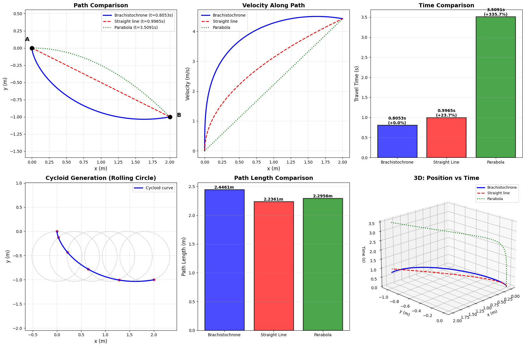
======================================================================
BRACHISTOCHRONE PROBLEM SOLUTION
======================================================================

Boundary Conditions:
  Start point A: (0.0, 0.0)
  End point B: (2.0, -1.0)
  Gravity: g = 9.8 m/s²

Cycloid Parameters:
  Radius r = 0.517200 m
  Maximum angle θ_max = 3.508369 rad = 201.01°

Path Type            Time (s)        Length (m)      Time Diff (%)  
----------------------------------------------------------------------
Brachistochrone      0.805323        2.446069        0.00% (optimal)
Straight Line        0.996476        2.236068        +23.74%        
Parabola             3.509062        2.295587        +335.73%       
======================================================================

Key Insight: The brachistochrone is 23.74% faster than
the straight line, even though it's 9.39% longer!
======================================================================

Physical Interpretation

The brachistochrone demonstrates a counterintuitive principle: the fastest path is not the shortest path. The cycloid dips down more steeply at the beginning, allowing the bead to gain velocity quickly. Even though this makes the path longer, the increased velocity more than compensates for the extra distance.

This problem has applications in:

  • Physics (particle trajectories)
  • Engineering (optimal ramp design)
  • Economics (optimal control theory)
  • Computer graphics (motion planning)

The cycloid curve appears naturally in many other contexts, including the tautochrone problem (where all particles reach the bottom in the same time, regardless of starting position) and in the design of gear teeth.