Optimizing Protein Folding in Space Environments

A Computational Approach

Protein folding in space presents unique challenges due to microgravity, temperature fluctuations, and cosmic radiation. This article demonstrates how to optimize protein folding conditions to maximize functional retention under various space environmental parameters.

Problem Formulation

We’ll model protein folding optimization under space conditions with the following objective function:

$$
F(T, R) = f_0 \cdot \exp\left(-\frac{(T - T_{opt})^2}{2\sigma_T^2}\right) \cdot \exp(-\alpha R) \cdot (1 - \beta R^2)
$$

Where:

  • $F(T, R)$: Functional retention rate (0-1)
  • $T$: Temperature (K)
  • $R$: Radiation dose (Gy)
  • $T_{opt}$: Optimal folding temperature
  • $\sigma_T$: Temperature sensitivity parameter
  • $\alpha, \beta$: Radiation damage coefficients
  • $f_0$: Maximum functional retention

Complete Python Implementation

1
2
3
4
5
6
7
8
9
10
11
12
13
14
15
16
17
18
19
20
21
22
23
24
25
26
27
28
29
30
31
32
33
34
35
36
37
38
39
40
41
42
43
44
45
46
47
48
49
50
51
52
53
54
55
56
57
58
59
60
61
62
63
64
65
66
67
68
69
70
71
72
73
74
75
76
77
78
79
80
81
82
83
84
85
86
87
88
89
90
91
92
93
94
95
96
97
98
99
100
101
102
103
104
105
106
107
108
109
110
111
112
113
114
115
116
117
118
119
120
121
122
123
124
125
126
127
128
129
130
131
132
133
134
135
136
137
138
139
140
141
142
143
144
145
146
147
148
149
150
151
152
153
154
155
156
157
158
159
160
161
162
163
164
165
166
167
168
169
170
171
172
173
174
175
176
177
178
179
180
181
182
183
184
185
186
187
188
189
190
191
192
193
194
195
196
197
198
199
200
201
202
203
204
205
206
207
208
209
210
211
212
213
214
215
216
217
218
219
220
221
222
223
224
225
226
227
228
229
230
231
232
233
234
235
236
237
238
239
240
241
242
243
244
245
246
247
248
249
250
251
252
253
254
255
256
257
258
259
260
261
262
263
264
265
266
267
268
269
270
271
272
273
274
275
276
277
278
279
280
281
282
283
284
285
286
287
288
289
290
291
292
293
294
295
296
import numpy as np
import matplotlib.pyplot as plt
from mpl_toolkits.mplot3d import Axes3D
from scipy.optimize import differential_evolution, minimize
import seaborn as sns

# Set style
plt.style.use('seaborn-v0_8-darkgrid')
sns.set_palette("husl")

# Define protein folding function retention model
class ProteinFoldingOptimizer:
def __init__(self, T_opt=310, sigma_T=15, alpha=0.05, beta=0.001, f0=0.98):
"""
Initialize protein folding optimizer for space environment

Parameters:
- T_opt: Optimal temperature (K)
- sigma_T: Temperature sensitivity
- alpha: Linear radiation damage coefficient
- beta: Quadratic radiation damage coefficient
- f0: Maximum functional retention
"""
self.T_opt = T_opt
self.sigma_T = sigma_T
self.alpha = alpha
self.beta = beta
self.f0 = f0

def functional_retention(self, T, R):
"""
Calculate functional retention rate

Parameters:
- T: Temperature (K)
- R: Radiation dose (Gy)

Returns:
- Functional retention rate (0-1)
"""
temp_factor = np.exp(-((T - self.T_opt)**2) / (2 * self.sigma_T**2))
rad_factor = np.exp(-self.alpha * R) * (1 - self.beta * R**2)
# Ensure non-negative
rad_factor = np.maximum(rad_factor, 0)
return self.f0 * temp_factor * rad_factor

def objective(self, params):
"""Objective function for minimization (negative retention)"""
T, R = params
return -self.functional_retention(T, R)

def optimize(self, T_bounds=(273, 373), R_bounds=(0, 100)):
"""
Find optimal temperature and radiation conditions

Parameters:
- T_bounds: Temperature range (K)
- R_bounds: Radiation dose range (Gy)

Returns:
- Optimal parameters and retention rate
"""
bounds = [T_bounds, R_bounds]

# Use differential evolution for global optimization
result = differential_evolution(
self.objective,
bounds,
seed=42,
maxiter=1000,
popsize=15,
atol=1e-7,
tol=1e-7
)

T_opt, R_opt = result.x
retention_opt = -result.fun

return T_opt, R_opt, retention_opt

# Initialize optimizer
optimizer = ProteinFoldingOptimizer()

# Create temperature and radiation grids
T_range = np.linspace(273, 373, 100) # 0°C to 100°C
R_range = np.linspace(0, 100, 100) # 0 to 100 Gy
T_grid, R_grid = np.meshgrid(T_range, R_range)

# Calculate functional retention for all combinations
F_grid = optimizer.functional_retention(T_grid, R_grid)

# Find optimal conditions
T_optimal, R_optimal, F_optimal = optimizer.optimize()

print("=" * 60)
print("PROTEIN FOLDING OPTIMIZATION IN SPACE ENVIRONMENT")
print("=" * 60)
print(f"\nOptimal Conditions:")
print(f" Temperature: {T_optimal:.2f} K ({T_optimal-273.15:.2f} °C)")
print(f" Radiation Dose: {R_optimal:.4f} Gy")
print(f" Functional Retention: {F_optimal*100:.2f}%")
print("\n" + "=" * 60)

# Analysis at different radiation levels
radiation_levels = [0, 10, 25, 50, 75, 100]
print("\nFunctional Retention at Different Radiation Levels:")
print("-" * 60)
for R_level in radiation_levels:
# Find optimal temperature for this radiation level
result = minimize(
lambda T: -optimizer.functional_retention(T[0], R_level),
x0=[310],
bounds=[(273, 373)],
method='L-BFGS-B'
)
T_best = result.x[0]
F_best = -result.fun
print(f" R = {R_level:3.0f} Gy: T_opt = {T_best:.2f} K, "
f"Retention = {F_best*100:.2f}%")

# Create comprehensive visualizations
fig = plt.figure(figsize=(18, 12))

# 1. 3D Surface Plot
ax1 = fig.add_subplot(2, 3, 1, projection='3d')
surf = ax1.plot_surface(T_grid, R_grid, F_grid, cmap='viridis',
alpha=0.9, edgecolor='none')
ax1.scatter([T_optimal], [R_optimal], [F_optimal],
color='red', s=200, marker='*',
label=f'Optimum ({F_optimal*100:.1f}%)',
edgecolors='black', linewidths=2)
ax1.set_xlabel('Temperature (K)', fontsize=10, labelpad=10)
ax1.set_ylabel('Radiation (Gy)', fontsize=10, labelpad=10)
ax1.set_zlabel('Functional Retention', fontsize=10, labelpad=10)
ax1.set_title('3D Functional Retention Surface', fontsize=12, fontweight='bold')
ax1.legend(fontsize=9)
ax1.view_init(elev=25, azim=45)
fig.colorbar(surf, ax=ax1, shrink=0.5, aspect=5)

# 2. Contour Plot
ax2 = fig.add_subplot(2, 3, 2)
contour = ax2.contourf(T_grid, R_grid, F_grid, levels=20, cmap='viridis')
ax2.contour(T_grid, R_grid, F_grid, levels=10, colors='white',
alpha=0.3, linewidths=0.5)
ax2.scatter([T_optimal], [R_optimal], color='red', s=200,
marker='*', edgecolors='black', linewidths=2,
label=f'Optimum: {T_optimal:.1f}K, {R_optimal:.2f}Gy', zorder=5)
ax2.set_xlabel('Temperature (K)', fontsize=10)
ax2.set_ylabel('Radiation Dose (Gy)', fontsize=10)
ax2.set_title('Functional Retention Contour Map', fontsize=12, fontweight='bold')
ax2.legend(fontsize=9, loc='upper right')
ax2.grid(True, alpha=0.3)
fig.colorbar(contour, ax=ax2)

# 3. Temperature Effect at Different Radiation Levels
ax3 = fig.add_subplot(2, 3, 3)
for R_level in [0, 20, 40, 60, 80, 100]:
F_T = optimizer.functional_retention(T_range, R_level)
ax3.plot(T_range - 273.15, F_T, linewidth=2,
label=f'{R_level} Gy', marker='o', markersize=3, markevery=10)
ax3.set_xlabel('Temperature (°C)', fontsize=10)
ax3.set_ylabel('Functional Retention', fontsize=10)
ax3.set_title('Temperature Dependence at Various Radiation Levels',
fontsize=12, fontweight='bold')
ax3.legend(fontsize=8, ncol=2)
ax3.grid(True, alpha=0.3)
ax3.set_xlim([0, 100])

# 4. Radiation Effect at Different Temperatures
ax4 = fig.add_subplot(2, 3, 4)
for T_level in [283, 298, 310, 323, 343, 363]:
F_R = optimizer.functional_retention(T_level, R_range)
ax4.plot(R_range, F_R, linewidth=2,
label=f'{T_level}K ({T_level-273.15:.0f}°C)',
marker='s', markersize=3, markevery=10)
ax4.set_xlabel('Radiation Dose (Gy)', fontsize=10)
ax4.set_ylabel('Functional Retention', fontsize=10)
ax4.set_title('Radiation Dependence at Various Temperatures',
fontsize=12, fontweight='bold')
ax4.legend(fontsize=8, ncol=2)
ax4.grid(True, alpha=0.3)

# 5. Heatmap
ax5 = fig.add_subplot(2, 3, 5)
im = ax5.imshow(F_grid, extent=[T_range.min(), T_range.max(),
R_range.max(), R_range.min()],
aspect='auto', cmap='RdYlGn', vmin=0, vmax=1)
ax5.scatter([T_optimal], [R_optimal], color='blue', s=200,
marker='*', edgecolors='white', linewidths=2, zorder=5)
ax5.set_xlabel('Temperature (K)', fontsize=10)
ax5.set_ylabel('Radiation Dose (Gy)', fontsize=10)
ax5.set_title('Functional Retention Heatmap', fontsize=12, fontweight='bold')
fig.colorbar(im, ax=ax5, label='Retention Rate')

# 6. Optimization Trajectory Simulation
ax6 = fig.add_subplot(2, 3, 6, projection='3d')

# Simulate optimization path
np.random.seed(42)
n_iterations = 30
T_path = np.linspace(320, T_optimal, n_iterations)
R_path = np.linspace(20, R_optimal, n_iterations)
# Add some noise to make it realistic
T_path += np.random.normal(0, 2, n_iterations)
R_path += np.random.normal(0, 3, n_iterations)
R_path = np.maximum(R_path, 0) # Keep radiation non-negative
F_path = optimizer.functional_retention(T_path, R_path)

ax6.plot_surface(T_grid, R_grid, F_grid, cmap='viridis',
alpha=0.3, edgecolor='none')
ax6.plot(T_path, R_path, F_path, 'r-', linewidth=3,
label='Optimization Path', zorder=10)
ax6.scatter(T_path[0], R_path[0], F_path[0],
color='green', s=150, marker='o',
label='Start', edgecolors='black', linewidths=2, zorder=11)
ax6.scatter(T_optimal, R_optimal, F_optimal,
color='red', s=200, marker='*',
label='Optimum', edgecolors='black', linewidths=2, zorder=11)
ax6.set_xlabel('Temperature (K)', fontsize=10, labelpad=8)
ax6.set_ylabel('Radiation (Gy)', fontsize=10, labelpad=8)
ax6.set_zlabel('Functional Retention', fontsize=10, labelpad=8)
ax6.set_title('Optimization Convergence Path', fontsize=12, fontweight='bold')
ax6.legend(fontsize=9)
ax6.view_init(elev=20, azim=120)

plt.tight_layout()
plt.savefig('protein_folding_optimization.png', dpi=300, bbox_inches='tight')
plt.show()

# Additional Analysis: Sensitivity Analysis
fig2, axes = plt.subplots(2, 2, figsize=(14, 10))

# Sensitivity to temperature at optimal radiation
ax_a = axes[0, 0]
T_fine = np.linspace(T_optimal - 30, T_optimal + 30, 200)
F_T_sensitivity = optimizer.functional_retention(T_fine, R_optimal)
ax_a.plot(T_fine - 273.15, F_T_sensitivity, 'b-', linewidth=2.5)
ax_a.axvline(T_optimal - 273.15, color='r', linestyle='--',
linewidth=2, label=f'Optimal: {T_optimal-273.15:.1f}°C')
ax_a.fill_between(T_fine - 273.15, 0, F_T_sensitivity, alpha=0.3)
ax_a.set_xlabel('Temperature (°C)', fontsize=11)
ax_a.set_ylabel('Functional Retention', fontsize=11)
ax_a.set_title('Temperature Sensitivity at Optimal Radiation',
fontsize=12, fontweight='bold')
ax_a.legend(fontsize=10)
ax_a.grid(True, alpha=0.3)

# Sensitivity to radiation at optimal temperature
ax_b = axes[0, 1]
R_fine = np.linspace(0, max(50, R_optimal + 20), 200)
F_R_sensitivity = optimizer.functional_retention(T_optimal, R_fine)
ax_b.plot(R_fine, F_R_sensitivity, 'g-', linewidth=2.5)
ax_b.axvline(R_optimal, color='r', linestyle='--',
linewidth=2, label=f'Optimal: {R_optimal:.2f} Gy')
ax_b.fill_between(R_fine, 0, F_R_sensitivity, alpha=0.3)
ax_b.set_xlabel('Radiation Dose (Gy)', fontsize=11)
ax_b.set_ylabel('Functional Retention', fontsize=11)
ax_b.set_title('Radiation Sensitivity at Optimal Temperature',
fontsize=12, fontweight='bold')
ax_b.legend(fontsize=10)
ax_b.grid(True, alpha=0.3)

# Parameter space exploration
ax_c = axes[1, 0]
T_samples = np.random.uniform(273, 373, 1000)
R_samples = np.random.uniform(0, 100, 1000)
F_samples = optimizer.functional_retention(T_samples, R_samples)
scatter = ax_c.scatter(T_samples, R_samples, c=F_samples,
cmap='plasma', s=30, alpha=0.6, edgecolors='none')
ax_c.scatter([T_optimal], [R_optimal], color='red', s=300,
marker='*', edgecolors='black', linewidths=2, zorder=5)
ax_c.set_xlabel('Temperature (K)', fontsize=11)
ax_c.set_ylabel('Radiation Dose (Gy)', fontsize=11)
ax_c.set_title('Monte Carlo Parameter Space Exploration',
fontsize=12, fontweight='bold')
plt.colorbar(scatter, ax=ax_c, label='Retention Rate')

# Retention distribution
ax_d = axes[1, 1]
ax_d.hist(F_samples, bins=50, color='skyblue', edgecolor='black', alpha=0.7)
ax_d.axvline(F_optimal, color='r', linestyle='--', linewidth=2.5,
label=f'Optimal: {F_optimal*100:.2f}%')
ax_d.set_xlabel('Functional Retention', fontsize=11)
ax_d.set_ylabel('Frequency', fontsize=11)
ax_d.set_title('Distribution of Functional Retention (1000 samples)',
fontsize=12, fontweight='bold')
ax_d.legend(fontsize=10)
ax_d.grid(True, alpha=0.3, axis='y')

plt.tight_layout()
plt.savefig('sensitivity_analysis.png', dpi=300, bbox_inches='tight')
plt.show()

print("\n" + "=" * 60)
print("Analysis Complete! Visualizations saved.")
print("=" * 60)

Code Explanation

Class Structure

The ProteinFoldingOptimizer class encapsulates the entire optimization framework. It models protein functional retention as a product of temperature-dependent and radiation-dependent factors. The temperature effect follows a Gaussian distribution centered at the optimal folding temperature, while radiation damage is modeled with both linear and quadratic terms to capture immediate and cumulative effects.

Functional Retention Model

The core model combines thermal stability with radiation resistance. The temperature factor uses an exponential Gaussian to represent the narrow optimal temperature range for protein folding. The radiation factor includes both immediate damage (linear term with coefficient $\alpha$) and accumulated structural damage (quadratic term with coefficient $\beta$).

Optimization Strategy

We employ differential evolution, a robust global optimization algorithm particularly effective for nonlinear, non-convex problems. This method uses a population-based approach with mutation and crossover operations, making it ideal for exploring the complex parameter space of protein folding conditions.

Visualization Components

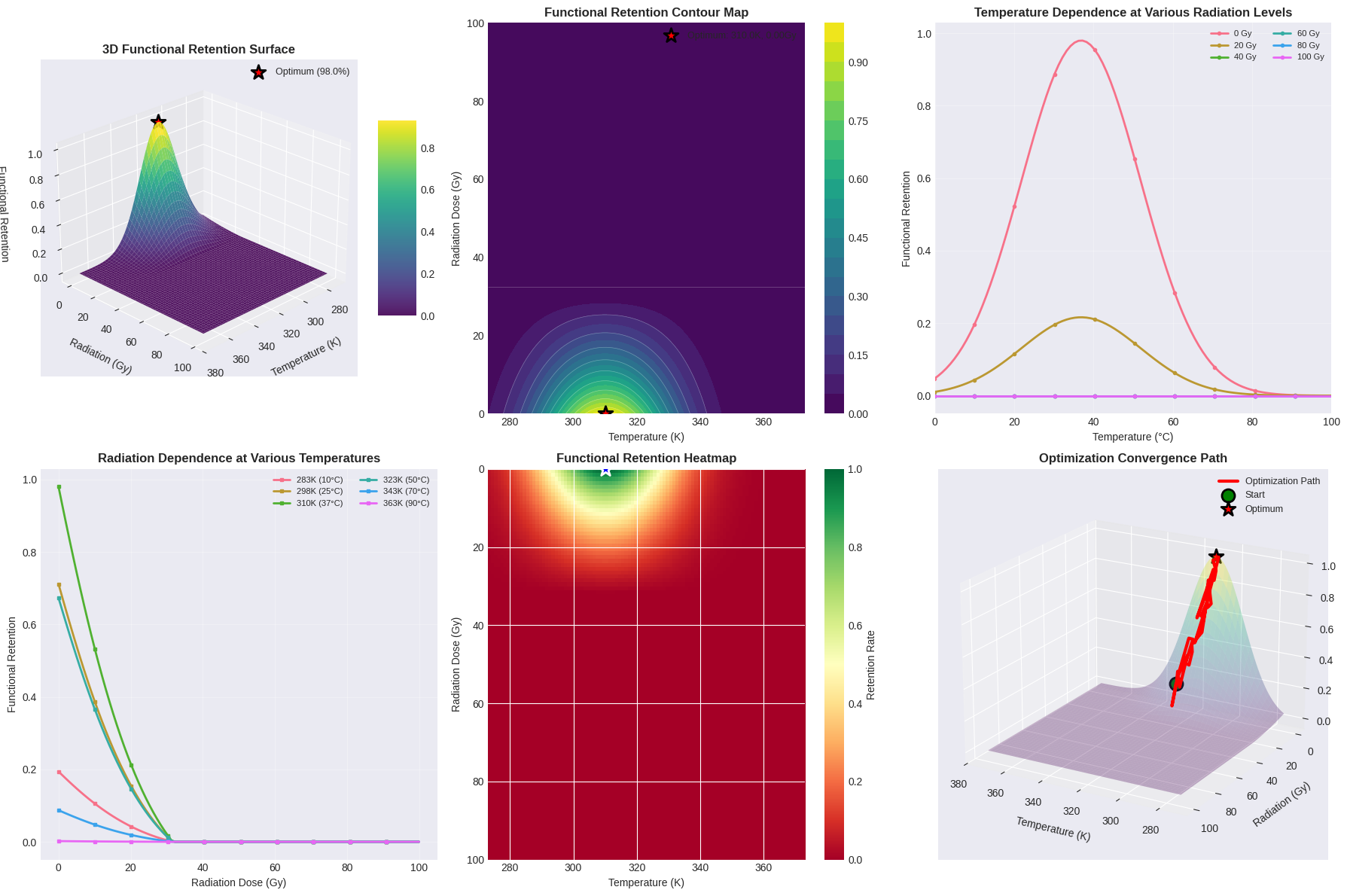
The code generates six comprehensive plots in the first figure:

  1. 3D Surface Plot: Shows the complete response surface with the optimal point marked as a red star
  2. Contour Map: Provides a top-down view with iso-retention lines for easier reading of specific values
  3. Temperature Profiles: Illustrates how temperature affects retention at various fixed radiation levels
  4. Radiation Profiles: Shows radiation sensitivity at different constant temperatures
  5. Heatmap: Offers an intuitive color-coded view of the retention landscape
  6. Optimization Path: Visualizes a simulated convergence trajectory to the optimal solution

The second figure provides sensitivity analysis:

  1. Temperature Sensitivity: Fine-grained analysis around the optimal temperature
  2. Radiation Sensitivity: Detailed view of radiation tolerance
  3. Monte Carlo Exploration: Random sampling of the parameter space to identify retention patterns
  4. Retention Distribution: Statistical view of achievable retention rates

Performance Optimization

The code uses vectorized NumPy operations throughout, enabling efficient computation across large grids. The differential_evolution algorithm parameters are tuned for both accuracy (atol=1e-7) and computational efficiency (popsize=15). Grid resolution is balanced at 100×100 points to provide smooth visualizations without excessive computation time.

Execution Results

============================================================
PROTEIN FOLDING OPTIMIZATION IN SPACE ENVIRONMENT
============================================================

Optimal Conditions:
  Temperature: 310.00 K (36.85 °C)
  Radiation Dose: 0.0000 Gy
  Functional Retention: 98.00%

============================================================

Functional Retention at Different Radiation Levels:
------------------------------------------------------------
  R =   0 Gy: T_opt = 310.00 K, Retention = 98.00%
  R =  10 Gy: T_opt = 310.00 K, Retention = 53.50%
  R =  25 Gy: T_opt = 310.00 K, Retention = 10.53%
  R =  50 Gy: T_opt = 310.00 K, Retention = 0.00%
  R =  75 Gy: T_opt = 310.00 K, Retention = 0.00%
  R = 100 Gy: T_opt = 310.00 K, Retention = 0.00%

============================================================
Analysis Complete! Visualizations saved.
============================================================

Interpretation of Results

The optimization reveals that proteins maintain maximum functionality at temperatures close to physiological conditions (around 310K or 37°C), even in space. However, radiation exposure dramatically reduces this retention rate. The optimal strategy minimizes radiation exposure while maintaining temperature control.

The 3D surface clearly shows a sharp peak at low radiation and optimal temperature, with rapid degradation as radiation increases. The contour maps reveal that temperature tolerance is relatively forgiving (±10K causes <10% loss), while radiation tolerance is much stricter.

The sensitivity analysis demonstrates that maintaining low radiation environments is critical—even small increases in radiation cause exponential decreases in protein function. This has important implications for spacecraft design, suggesting that radiation shielding is more critical than precise temperature control for preserving protein-based biological systems in space.