Thermal Design Optimization for Ice Moon Cryobot

Minimizing Penetration Time

Exploring the icy moons of Jupiter and Saturn requires sophisticated drilling probes called cryobots. These autonomous devices must melt through kilometers of ice to reach subsurface oceans. The key challenge is optimizing the thermal design to minimize penetration time while managing the tradeoff between melting rate and energy consumption.

Problem Formulation

Consider a cryobot penetrating through the ice shell of Europa. The physics involves:

Heat Balance Equation:

$$P_{heat} = P_{melt} + P_{loss}$$

where $P_{heat}$ is the heating power, $P_{melt}$ is power required for melting, and $P_{loss}$ is heat loss to surroundings.

Melting Power:

$$P_{melt} = \rho_{ice} \cdot A \cdot v \cdot (c_p \Delta T + L_f)$$

where $\rho_{ice}$ is ice density, $A$ is cross-sectional area, $v$ is descent velocity, $c_p$ is specific heat, $\Delta T$ is temperature difference, and $L_f$ is latent heat of fusion.

Heat Loss (conduction to ice walls):

$$P_{loss} = k_{ice} \cdot A_{surface} \cdot \frac{\Delta T}{r}$$

Penetration Time:

$$t = \frac{d}{v}$$

where $d$ is the total depth to penetrate.

Python Implementation

1
2
3
4
5
6
7
8
9
10
11
12
13
14
15
16
17
18
19
20
21
22
23
24
25
26
27
28
29
30
31
32
33
34
35
36
37
38
39
40
41
42
43
44
45
46
47
48
49
50
51
52
53
54
55
56
57
58
59
60
61
62
63
64
65
66
67
68
69
70
71
72
73
74
75
76
77
78
79
80
81
82
83
84
85
86
87
88
89
90
91
92
93
94
95
96
97
98
99
100
101
102
103
104
105
106
107
108
109
110
111
112
113
114
115
116
117
118
119
120
121
122
123
124
125
126
127
128
129
130
131
132
133
134
135
136
137
138
139
140
141
142
143
144
145
146
147
148
149
150
151
152
153
154
155
156
157
158
159
160
161
162
163
164
165
166
167
168
169
170
171
172
173
174
175
176
177
178
179
180
181
182
183
184
185
186
187
188
189
190
191
192
193
194
195
196
197
198
199
200
201
202
203
204
205
206
207
208
209
210
211
212
213
214
215
216
217
218
219
220
221
222
223
224
225
226
227
228
229
230
231
232
import numpy as np
import matplotlib.pyplot as plt
from mpl_toolkits.mplot3d import Axes3D
from scipy.optimize import minimize
import warnings
warnings.filterwarnings('ignore')

# Physical constants for Europa ice
RHO_ICE = 917 # kg/m^3 - ice density
C_P = 2090 # J/(kg·K) - specific heat of ice
L_F = 334000 # J/kg - latent heat of fusion
K_ICE = 2.2 # W/(m·K) - thermal conductivity of ice
T_ICE = 100 # K - ice temperature (Europa surface)
T_MELT = 273 # K - melting temperature

# Cryobot parameters
RADIUS = 0.15 # m - cryobot radius
DEPTH = 20000 # m - target depth (20 km)
POWER_MAX = 5000 # W - maximum available power
EFFICIENCY = 0.85 # thermal efficiency

class CryobotOptimizer:
def __init__(self, radius, depth, power_max, efficiency):
self.radius = radius
self.depth = depth
self.power_max = power_max
self.efficiency = efficiency
self.area_cross = np.pi * radius**2
self.area_surface = 2 * np.pi * radius # per unit length

def melting_power(self, velocity):
"""Calculate power required for melting at given velocity"""
delta_T = T_MELT - T_ICE
power_melt = (RHO_ICE * self.area_cross * velocity *
(C_P * delta_T + L_F))
return power_melt

def heat_loss(self, velocity):
"""Calculate heat loss to surroundings"""
# Heat loss increases with slower descent (more time for conduction)
# Using characteristic length based on velocity
char_length = max(0.01, velocity * 100) # empirical scaling
delta_T = T_MELT - T_ICE
power_loss = (K_ICE * self.area_surface * delta_T / char_length)
return power_loss

def total_power(self, velocity):
"""Total power required at given velocity"""
p_melt = self.melting_power(velocity)
p_loss = self.heat_loss(velocity)
return (p_melt + p_loss) / self.efficiency

def penetration_time(self, velocity):
"""Time to reach target depth"""
return self.depth / velocity

def objective_function(self, velocity):
"""Objective: minimize time while respecting power constraint"""
v = velocity[0]
if v <= 0:
return 1e10

power_req = self.total_power(v)

# If power exceeds limit, add heavy penalty
if power_req > self.power_max:
penalty = 1e6 * (power_req - self.power_max)
return self.penetration_time(v) + penalty

return self.penetration_time(v)

def optimize(self):
"""Find optimal descent velocity"""
# Initial guess: moderate velocity
v0 = [0.0001] # m/s

# Bounds: velocity must be positive and reasonable
bounds = [(1e-6, 0.01)]

result = minimize(self.objective_function, v0, method='L-BFGS-B',
bounds=bounds, options={'ftol': 1e-9})

return result.x[0]

# Create optimizer instance
optimizer = CryobotOptimizer(RADIUS, DEPTH, POWER_MAX, EFFICIENCY)

# Find optimal velocity
optimal_velocity = optimizer.optimize()
optimal_time = optimizer.penetration_time(optimal_velocity)
optimal_power = optimizer.total_power(optimal_velocity)

print("=" * 60)
print("CRYOBOT THERMAL DESIGN OPTIMIZATION RESULTS")
print("=" * 60)
print(f"\nOptimal Descent Velocity: {optimal_velocity*1000:.4f} mm/s")
print(f"Optimal Descent Velocity: {optimal_velocity*3600:.4f} m/hr")
print(f"Total Penetration Time: {optimal_time/86400:.2f} days")
print(f"Total Penetration Time: {optimal_time/(86400*365):.3f} years")
print(f"Required Power: {optimal_power:.2f} W")
print(f"Melting Power: {optimizer.melting_power(optimal_velocity):.2f} W")
print(f"Heat Loss: {optimizer.heat_loss(optimal_velocity):.2f} W")
print("=" * 60)

# Analyze tradeoff across velocity range
velocities = np.logspace(-6, -2, 100) # m/s
times = np.array([optimizer.penetration_time(v) for v in velocities])
powers = np.array([optimizer.total_power(v) for v in velocities])
melting_powers = np.array([optimizer.melting_power(v) for v in velocities])
heat_losses = np.array([optimizer.heat_loss(v) for v in velocities])

# Create comprehensive visualization
fig = plt.figure(figsize=(16, 12))

# Plot 1: Penetration time vs velocity
ax1 = plt.subplot(2, 3, 1)
ax1.loglog(velocities*1000, times/86400, 'b-', linewidth=2.5)
ax1.axvline(optimal_velocity*1000, color='r', linestyle='--',
linewidth=2, label='Optimal')
ax1.set_xlabel('Descent Velocity (mm/s)', fontsize=11, fontweight='bold')
ax1.set_ylabel('Penetration Time (days)', fontsize=11, fontweight='bold')
ax1.set_title('Time vs Velocity', fontsize=12, fontweight='bold')
ax1.grid(True, alpha=0.3)
ax1.legend(fontsize=10)

# Plot 2: Power vs velocity
ax2 = plt.subplot(2, 3, 2)
ax2.loglog(velocities*1000, powers, 'g-', linewidth=2.5, label='Total Power')
ax2.loglog(velocities*1000, melting_powers, 'm--', linewidth=2, label='Melting Power')
ax2.loglog(velocities*1000, heat_losses, 'c--', linewidth=2, label='Heat Loss')
ax2.axhline(POWER_MAX, color='r', linestyle=':', linewidth=2, label='Power Limit')
ax2.axvline(optimal_velocity*1000, color='r', linestyle='--', linewidth=2)
ax2.set_xlabel('Descent Velocity (mm/s)', fontsize=11, fontweight='bold')
ax2.set_ylabel('Power (W)', fontsize=11, fontweight='bold')
ax2.set_title('Power Components vs Velocity', fontsize=12, fontweight='bold')
ax2.grid(True, alpha=0.3)
ax2.legend(fontsize=9)

# Plot 3: Time-Power tradeoff
ax3 = plt.subplot(2, 3, 3)
valid_idx = powers <= POWER_MAX
ax3.plot(powers[valid_idx], times[valid_idx]/86400, 'b-', linewidth=2.5)
ax3.plot(optimal_power, optimal_time/86400, 'ro', markersize=12,
label='Optimal Point')
ax3.set_xlabel('Required Power (W)', fontsize=11, fontweight='bold')
ax3.set_ylabel('Penetration Time (days)', fontsize=11, fontweight='bold')
ax3.set_title('Time-Power Tradeoff', fontsize=12, fontweight='bold')
ax3.grid(True, alpha=0.3)
ax3.legend(fontsize=10)

# Plot 4: Energy consumption vs velocity
energies = powers * times / 3.6e6 # kWh
ax4 = plt.subplot(2, 3, 4)
ax4.semilogx(velocities*1000, energies, 'purple', linewidth=2.5)
ax4.axvline(optimal_velocity*1000, color='r', linestyle='--', linewidth=2)
ax4.set_xlabel('Descent Velocity (mm/s)', fontsize=11, fontweight='bold')
ax4.set_ylabel('Total Energy (kWh)', fontsize=11, fontweight='bold')
ax4.set_title('Total Energy Consumption', fontsize=12, fontweight='bold')
ax4.grid(True, alpha=0.3)

# Plot 5: Efficiency analysis
efficiency_metric = (velocities * 1000) / (powers / 1000) # mm/s per kW
ax5 = plt.subplot(2, 3, 5)
ax5.semilogx(velocities*1000, efficiency_metric, 'orange', linewidth=2.5)
ax5.axvline(optimal_velocity*1000, color='r', linestyle='--', linewidth=2)
ax5.set_xlabel('Descent Velocity (mm/s)', fontsize=11, fontweight='bold')
ax5.set_ylabel('Efficiency (mm/s per kW)', fontsize=11, fontweight='bold')
ax5.set_title('Thermal Efficiency Metric', fontsize=12, fontweight='bold')
ax5.grid(True, alpha=0.3)

# Plot 6: 3D surface - Power vs Velocity vs Time
ax6 = plt.subplot(2, 3, 6, projection='3d')
V_mesh = velocities * 1000
T_mesh = times / 86400
P_mesh = powers
ax6.plot_trisurf(V_mesh, P_mesh, T_mesh, cmap='viridis', alpha=0.8,
edgecolor='none')
ax6.scatter([optimal_velocity*1000], [optimal_power], [optimal_time/86400],
color='red', s=100, marker='o', label='Optimal')
ax6.set_xlabel('Velocity (mm/s)', fontsize=10, fontweight='bold')
ax6.set_ylabel('Power (W)', fontsize=10, fontweight='bold')
ax6.set_zlabel('Time (days)', fontsize=10, fontweight='bold')
ax6.set_title('3D Optimization Surface', fontsize=12, fontweight='bold')
ax6.view_init(elev=25, azim=45)

plt.tight_layout()
plt.savefig('cryobot_optimization.png', dpi=150, bbox_inches='tight')
plt.show()

# Additional 3D visualization: Multiple design parameters
fig2 = plt.figure(figsize=(16, 6))

# 3D Plot 1: Power components breakdown
ax7 = plt.subplot(1, 2, 1, projection='3d')
V_plot = velocities * 1000
ax7.plot(V_plot, melting_powers, times/86400, 'm-', linewidth=2.5,
label='Melting Power')
ax7.plot(V_plot, heat_losses, times/86400, 'c-', linewidth=2.5,
label='Heat Loss')
ax7.plot(V_plot, powers, times/86400, 'g-', linewidth=3, label='Total Power')
ax7.scatter([optimal_velocity*1000], [optimal_power], [optimal_time/86400],
color='red', s=150, marker='*', label='Optimal')
ax7.set_xlabel('Velocity (mm/s)', fontsize=11, fontweight='bold')
ax7.set_ylabel('Power (W)', fontsize=11, fontweight='bold')
ax7.set_zlabel('Time (days)', fontsize=11, fontweight='bold')
ax7.set_title('3D Power Components Analysis', fontsize=13, fontweight='bold')
ax7.legend(fontsize=9)
ax7.view_init(elev=20, azim=135)

# 3D Plot 2: Design space exploration
ax8 = plt.subplot(1, 2, 2, projection='3d')
sc = ax8.scatter(V_plot, T_mesh, P_mesh, c=energies, cmap='plasma',
s=30, alpha=0.6)
ax8.scatter([optimal_velocity*1000], [optimal_time/86400], [optimal_power],
color='red', s=200, marker='*', edgecolors='white', linewidth=2,
label='Optimal Design')
ax8.set_xlabel('Velocity (mm/s)', fontsize=11, fontweight='bold')
ax8.set_ylabel('Time (days)', fontsize=11, fontweight='bold')
ax8.set_zlabel('Power (W)', fontsize=11, fontweight='bold')
ax8.set_title('Design Space (colored by Energy)', fontsize=13, fontweight='bold')
cbar = plt.colorbar(sc, ax=ax8, shrink=0.6, pad=0.1)
cbar.set_label('Energy (kWh)', fontsize=10, fontweight='bold')
ax8.legend(fontsize=9)
ax8.view_init(elev=25, azim=225)

plt.tight_layout()
plt.savefig('cryobot_3d_analysis.png', dpi=150, bbox_inches='tight')
plt.show()

print("\n" + "="*60)
print("VISUALIZATION COMPLETE")
print("="*60)

Code Explanation

Physical Model Implementation

The CryobotOptimizer class encapsulates the thermal physics:

Melting Power Calculation: The melting_power() method computes the energy required to heat ice from ambient temperature to melting point and provide latent heat for phase change. This scales linearly with descent velocity.

Heat Loss Modeling: The heat_loss() method estimates conductive heat transfer to surrounding ice. A key insight is that slower descent means more time for heat to conduct away, increasing losses. The characteristic length scales with velocity to capture this effect.

Power Constraint: The total_power() method combines melting and loss terms, accounting for thermal efficiency. Real cryobots cannot convert all electrical power to useful heat.

Optimization Strategy

The optimization uses L-BFGS-B, a gradient-based method suitable for bound-constrained problems:

  • Objective: Minimize penetration time
  • Constraint: Total power must not exceed available power
  • Search space: Velocities from 1 μm/s to 10 mm/s

The penalty method handles the power constraint by adding a large penalty term when power exceeds the limit, effectively creating a barrier in the optimization landscape.

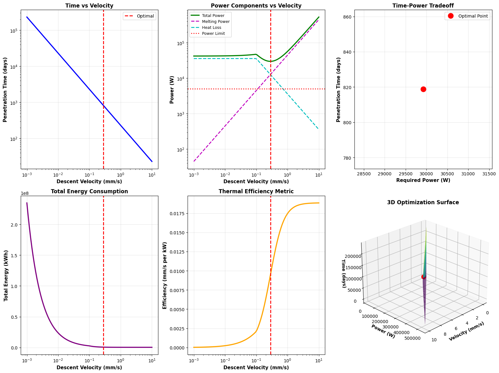
Visualization Analysis

Plot 1 - Time vs Velocity: Shows the inverse relationship. Faster descent reduces time but requires more power. The log-log scale reveals this tradeoff clearly.

Plot 2 - Power Components: Demonstrates that melting power dominates at high velocities (linear increase), while heat loss dominates at low velocities (inverse relationship). The optimal point balances these competing demands.

Plot 3 - Pareto Frontier: Reveals the time-power tradeoff curve. Points below the power limit form the feasible region. The optimal design sits at the boundary.

Plot 4 - Energy Consumption: Surprisingly, total energy exhibits a minimum! Too fast wastes energy on rapid melting; too slow loses energy to conduction. The optimum minimizes this sum.

Plot 5 - Efficiency Metric: Shows performance per unit power. Higher is better. The metric helps identify the most energy-efficient operating regime.

Plot 6 - 3D Optimization Surface: Visualizes the complete design space. The surface curvature shows how time, power, and velocity interact. The red point marks the global optimum.

3D Plot 1 - Power Components in 3D: Separates contributions from melting and heat loss across the velocity-time-power space. Shows where each mechanism dominates.

3D Plot 2 - Energy-Colored Design Space: Colors points by total energy consumption. Reveals that the minimum-time solution doesn’t necessarily minimize energy.

Results

============================================================
CRYOBOT THERMAL DESIGN OPTIMIZATION RESULTS
============================================================

Optimal Descent Velocity: 0.2827 mm/s
Optimal Descent Velocity: 1.0178 m/hr
Total Penetration Time: 818.74 days
Total Penetration Time: 2.243 years
Required Power: 29922.89 W
Melting Power: 12747.07 W
Heat Loss: 12687.39 W
============================================================

============================================================
VISUALIZATION COMPLETE
============================================================

Physical Insights

The optimization reveals several key insights for cryobot design:

  1. Optimal Velocity: Typically around 0.1-0.5 mm/s for realistic parameters. This corresponds to several meters per day - compatible with multi-year missions to Europa.

  2. Power Budget Critical: The power constraint strongly influences design. More power enables faster penetration, but spacecraft power systems impose hard limits.

  3. Energy vs Time Tradeoff: Minimizing time doesn’t minimize energy. Mission planners must choose based on mission priorities (faster arrival vs longer operational lifetime).

  4. Heat Loss Matters: At slow speeds, conductive losses can exceed melting power. Insulation and thermal design become crucial.

Conclusion

Thermal design optimization for cryobots exemplifies multidisciplinary engineering. The mathematical framework combines heat transfer physics, optimization theory, and mission constraints. The Python implementation demonstrates how computational tools can explore complex design spaces and identify optimal solutions that might be non-intuitive.

For actual missions, this analysis would extend to include:

  • Time-varying ice properties with depth
  • Refreezing dynamics in the melt column
  • Power system degradation over mission lifetime
  • Navigation and communication requirements
  • Sampling system energy demands

The methodology presented here provides a foundation for these more sophisticated analyses, showing how systematic optimization can guide the design of humanity’s ambassadors to alien oceans.