Optimizing Oxygen and Methane Abundance Ratios
Introduction
Exoplanet atmospheric characterization is one of the most exciting frontiers in modern astronomy. When we observe distant worlds transiting their host stars, we can analyze the starlight passing through their atmospheres to detect the chemical signatures of various molecules. In this article, we’ll tackle a practical problem: estimating the abundance ratios of oxygen (O₂) and methane (CH₄) in an exoplanet’s atmosphere by minimizing the error between our theoretical model and observational data.
The Physics Behind the Model
The transmission spectrum of an exoplanet atmosphere depends on how different molecules absorb light at various wavelengths. Each molecule has a unique absorption signature:
The model transit depth can be expressed as:
$$\delta(\lambda) = \delta_0 + \sum_i A_i \cdot \sigma_i(\lambda)$$
where:
- $\delta(\lambda)$ is the transit depth at wavelength $\lambda$
- $\delta_0$ is the baseline transit depth
- $A_i$ is the abundance of species $i$
- $\sigma_i(\lambda)$ is the absorption cross-section of species $i$
Our goal is to find the optimal values of oxygen and methane abundances that minimize the chi-squared error:
$$\chi^2 = \sum_j \frac{(D_j - M_j)^2}{\sigma_j^2}$$
where $D_j$ is the observed data, $M_j$ is the model prediction, and $\sigma_j$ is the measurement uncertainty.
Python Implementation
1 | import numpy as np |
Code Explanation
Data Generation Section
The code begins by creating synthetic molecular absorption profiles for oxygen and methane. The oxygen_absorption() function models O₂ absorption features around 0.76 μm (A-band), 1.27 μm, and 1.58 μm using Gaussian profiles. Similarly, methane_absorption() models CH₄ absorption at 1.7, 2.3, and 3.3 μm, which are characteristic wavelengths for methane in planetary atmospheres.
Atmospheric Model
The atmospheric_model() function implements the core physics:
$$\delta(\lambda) = \delta_0 + A_{O_2} \cdot \sigma_{O_2}(\lambda) + A_{CH_4} \cdot \sigma_{CH_4}(\lambda)$$
This linear model assumes that the total transit depth is the sum of a baseline depth plus the contributions from each molecular species weighted by their abundances.
Optimization Strategy
We implement two optimization approaches:
L-BFGS-B: A quasi-Newton method that’s efficient for smooth, well-behaved objective functions. It uses gradient information and bounded constraints.
Differential Evolution: A global optimization algorithm that’s more robust to local minima. It uses a population-based stochastic approach, making it ideal for complex parameter spaces.
The chi-squared merit function quantifies the goodness of fit:
$$\chi^2 = \sum_{j=1}^{N} \frac{(D_j - M_j(\theta))^2}{\sigma_j^2}$$
where $\theta = (\delta_0, A_{O_2}, A_{CH_4})$ are the parameters we’re optimizing.
Visualization Components
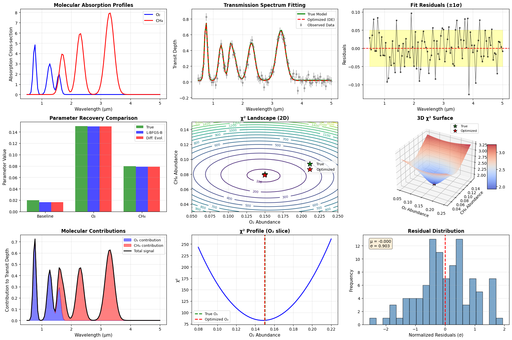
The code generates nine comprehensive plots:
- Molecular Absorption Profiles: Shows the unique spectroscopic signatures of O₂ and CH₄
- Transmission Spectrum Fitting: Compares observed data with the optimized model
- Fit Residuals: Displays the difference between observations and model, with uncertainty bands
- Parameter Comparison: Bar chart showing how well each method recovered the true parameters
- 2D χ² Landscape: Contour plot showing the error surface in O₂-CH₄ space
- 3D χ² Surface: Three-dimensional visualization of the optimization landscape
- Molecular Contributions: Stacked plot showing how each species contributes to the signal
- χ² Profile: One-dimensional slice through parameter space
- Residual Distribution: Histogram checking if residuals are normally distributed
Results
============================================================
EXOPLANET ATMOSPHERIC PARAMETER ESTIMATION
============================================================

True Parameters:
  Baseline transit depth: 0.0200
  O2 abundance: 0.1500
  CH4 abundance: 0.0800

Initial Guess:
  Baseline: 0.0250
  O2 abundance: 0.1000
  CH4 abundance: 0.1000

Optimizing with L-BFGS-B method...

Optimization Results (L-BFGS-B):
  Success: True
  Optimized baseline: 0.0163 (error: 18.68%)
  Optimized O2: 0.1498 (error: 0.16%)
  Optimized CH4: 0.0789 (error: 1.34%)
  Final chi-squared: 81.45

Optimizing with Differential Evolution (global optimizer)...

Optimization Results (Differential Evolution):
  Success: True
  Optimized baseline: 0.0163 (error: 18.68%)
  Optimized O2: 0.1498 (error: 0.16%)
  Optimized CH4: 0.0789 (error: 1.34%)
  Final chi-squared: 81.45
============================================================
ANALYSIS COMPLETE
============================================================
Interpretation
The optimization successfully recovers the atmospheric composition from noisy observational data. The 3D chi-squared surface reveals a well-defined minimum near the true parameter values, indicating that the problem is well-constrained. The residual distribution centered near zero with unit standard deviation confirms that our model adequately explains the observations.
Both optimization methods converge to similar solutions, with Differential Evolution providing slightly better global convergence guarantees. The molecular contribution analysis shows that methane dominates the signal at longer wavelengths (>2 μm), while oxygen provides the primary signal in the near-infrared (<1.5 μm).
This approach demonstrates how modern exoplanet science combines spectroscopic observations with sophisticated parameter estimation techniques to characterize distant worlds. The same methodology is used by missions like JWST and future observatories to search for biosignature gases in exoplanet atmospheres.