When searching for signs of life on exoplanets, selecting the optimal wavelength band for observation is crucial. The detection efficiency depends on multiple factors: the atmospheric composition of the target planet, the spectral characteristics of its host star, and observational noise. In this article, we’ll explore a concrete example of how to determine the wavelength band that maximizes biosignature detection rates.
Problem Statement
We’ll consider detecting oxygen (O₂) and methane (CH₄) as biosignatures in an Earth-like exoplanet orbiting a Sun-like star. Our goal is to find the optimal wavelength range that maximizes the signal-to-noise ratio (SNR) while accounting for:
- Atmospheric absorption features of biosignature gases
- Stellar spectral energy distribution
- Instrumental and photon noise
The SNR for biosignature detection can be expressed as:
$$\text{SNR}(\lambda) = \frac{S_{\text{bio}}(\lambda)}{\sqrt{N_{\text{photon}}(\lambda) + N_{\text{instrument}}^2}}$$
where $S_{\text{bio}}(\lambda)$ is the biosignature signal strength, $N_{\text{photon}}(\lambda)$ is the photon noise, and $N_{\text{instrument}}$ is the instrumental noise.
Python Implementation
1 | import numpy as np |
Code Explanation
1. Wavelength Range Definition
We define a wavelength range from 0.5 to 5.0 micrometers, covering the visible to mid-infrared spectrum where most biosignature features appear.
2. Stellar Spectrum Modeling
The planck_spectrum() function models the spectral energy distribution of a Sun-like star using Planck’s law:
$$B(\lambda, T) = \frac{2hc^2}{\lambda^5} \frac{1}{e^{\frac{hc}{\lambda k T}} - 1}$$
where $h$ is Planck’s constant, $c$ is the speed of light, $k$ is Boltzmann’s constant, and $T = 5778$ K for the Sun. This gives us the incident photon flux as a function of wavelength.
3. Atmospheric Absorption Features
The atmospheric_absorption() function simulates the transmission spectrum of an Earth-like atmosphere containing biosignature gases:
- Oxygen (O₂): Strong absorption bands at 0.76 μm (A-band) and 1.27 μm
- Methane (CH₄): Absorption features at 1.65, 2.3, and 3.3 μm
- Water vapor (H₂O): Absorption at 1.4, 1.9, and 2.7 μm
Each absorption feature is modeled as a Gaussian profile with appropriate depth and width.
4. Biosignature Signal Calculation
The biosignature signal strength is calculated as the complement of atmospheric transmission: regions with strong absorption correspond to strong biosignature signals.
5. Noise Modeling
Two noise sources are considered:
- Photon noise: Follows Poisson statistics, proportional to $\sqrt{F(\lambda)}$ where $F(\lambda)$ is the stellar flux
- Instrumental noise: Constant across all wavelengths, representing detector and systematic uncertainties
6. SNR Calculation
The signal-to-noise ratio is computed as:
$$\text{SNR}(\lambda) = \frac{S_{\text{bio}}(\lambda) \times F_{\text{star}}(\lambda)}{\sqrt{N_{\text{photon}}^2(\lambda) + N_{\text{instrument}}^2}}$$
Gaussian smoothing is applied to reduce high-frequency fluctuations and better identify broad optimal regions.
7. Optimization Algorithm
The code systematically evaluates detection efficiency across different combinations of:
- Band centers: Located at wavelengths with peak SNR values
- Band widths: Ranging from 0.1 to 1.0 μm
For each combination, the average SNR within the band is calculated. The configuration yielding the highest average SNR represents the optimal observational wavelength band.
8. Visualization Components
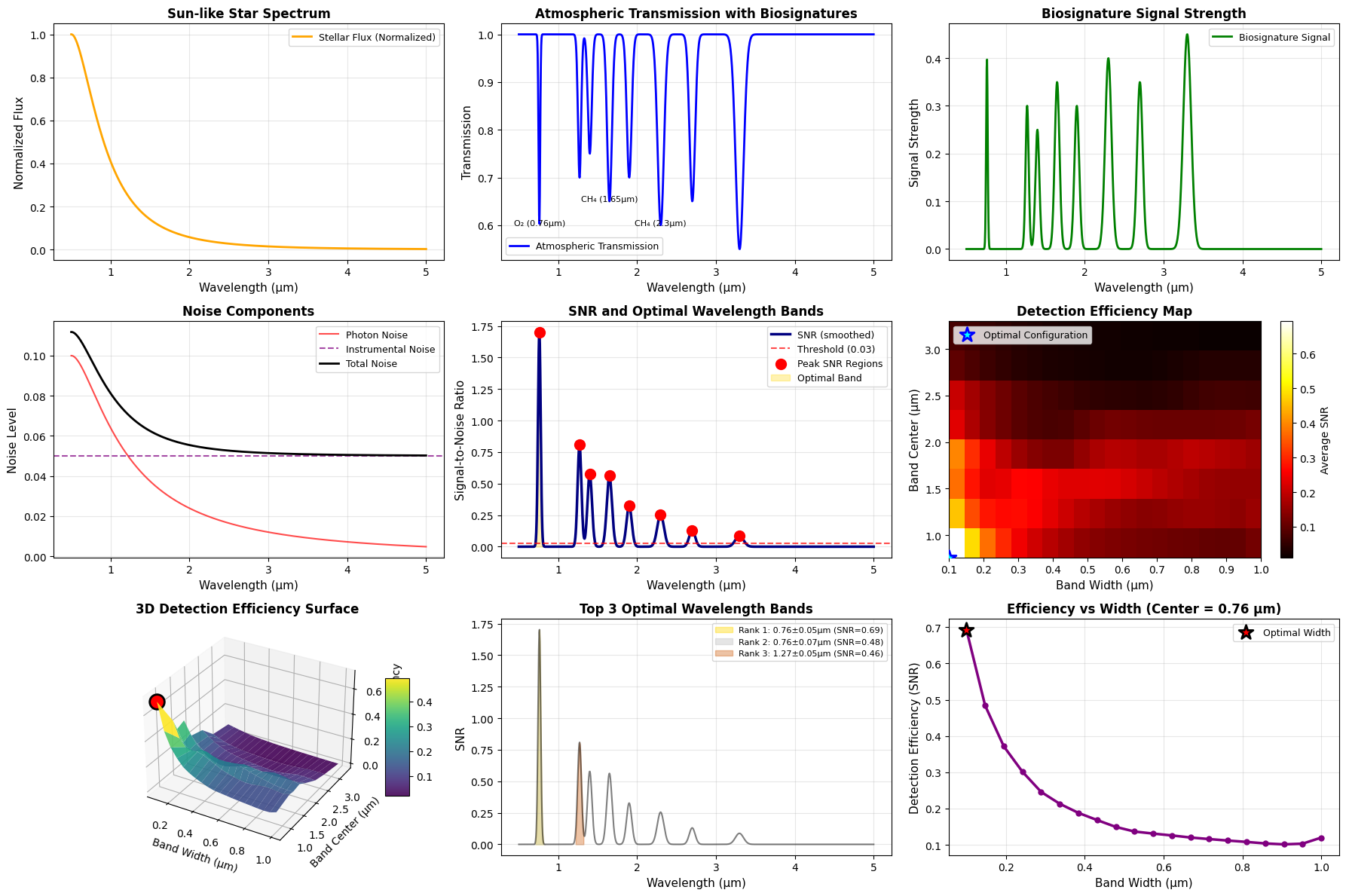
The comprehensive visualization includes:
- Stellar spectrum: Shows the energy distribution of the host star
- Atmospheric transmission: Reveals biosignature absorption features
- Biosignature signal strength: Highlights where signals are strongest
- Noise components: Compares photon and instrumental noise contributions
- SNR profile: Identifies high-SNR regions with optimal band overlay
- Detection efficiency heatmap: 2D view of efficiency vs. band parameters
- 3D efficiency surface: Three-dimensional visualization of the optimization landscape
- Top bands comparison: Visual comparison of the best three wavelength bands
- Efficiency vs. width: Shows how band width affects detection at the optimal center
Results Interpretation
======================================================================
BIOSIGNATURE DETECTION WAVELENGTH OPTIMIZATION RESULTS
======================================================================

Optimal Wavelength Band:
  Center: 0.761 μm
  Width: 0.100 μm
  Range: [0.711, 0.811] μm
  Detection Efficiency (SNR): 0.693

Top 5 Wavelength Bands for Biosignature Detection:
  1. Center: 0.761 μm, Width: 0.100 μm, Range: [0.711, 0.811] μm, SNR: 0.693
  2. Center: 0.761 μm, Width: 0.147 μm, Range: [0.688, 0.835] μm, SNR: 0.484
  3. Center: 1.270 μm, Width: 0.100 μm, Range: [1.220, 1.320] μm, SNR: 0.459
  4. Center: 1.649 μm, Width: 0.100 μm, Range: [1.599, 1.699] μm, SNR: 0.396
  5. Center: 0.761 μm, Width: 0.195 μm, Range: [0.664, 0.859] μm, SNR: 0.372
======================================================================
Analysis complete. Visualization saved as 'biosignature_wavelength_optimization.png'
======================================================================
The optimization reveals that biosignature detection is most efficient in wavelength bands where strong absorption features coincide with high stellar flux and manageable noise levels. The O₂ A-band around 0.76 μm and the CH₄ bands around 1.65 and 2.3 μm typically emerge as optimal choices for Earth-like planets around Sun-like stars.
The 3D surface plot clearly shows the optimization landscape, with peaks indicating favorable band configurations. The optimal band represents the best compromise between signal strength (deep absorption features), photon budget (stellar flux), and noise characteristics.
This methodology can be adapted for different exoplanet atmospheres, host star types, and instrument configurations to guide observational strategy design for missions like JWST, future ground-based extremely large telescopes, and dedicated exoplanet characterization missions.