Optimizing the Habitable Zone

January 22, 2026

Maximizing Liquid Water Duration

The habitable zone (HZ) is the region around a star where liquid water can exist on a planetary surface. The duration of this favorable condition depends on stellar mass, age, and metallicity. Let’s explore this optimization problem through a concrete example.

Problem Definition

We want to find the optimal stellar parameters that maximize the duration of liquid water existence in the habitable zone. The key relationships are:

Stellar Luminosity Evolution:
$$L(t) = L_0 \left(1 + \frac{t}{t_{MS}}\right)$$

Main Sequence Lifetime:
$$t_{MS} = 10 \times \left(\frac{M}{M_{\odot}}\right)^{-2.5} \text{ Gyr}$$

Habitable Zone Boundaries:
$$d_{inner} = \sqrt{\frac{L}{1.1}} \text{ AU}, \quad d_{outer} = \sqrt{\frac{L}{0.53}} \text{ AU}$$

Metallicity Effect:
The metallicity [Fe/H] affects both luminosity and main sequence lifetime through empirical corrections.

Python Implementation

import numpy as np
import matplotlib.pyplot as plt
from mpl_toolkits.mplot3d import Axes3D
from scipy.optimize import differential_evolution
import warnings
import os
warnings.filterwarnings('ignore')

# 出力ディレクトリの作成
os.makedirs('/mnt/user-data/outputs', exist_ok=True)

# 定数定義
SOLAR_MASS = 1.0
SOLAR_LUMINOSITY = 1.0

class HabitableZoneOptimizer:
    """生命居住可能領域の最適化クラス"""
    
    def __init__(self):
        self.results = {}
    
    def stellar_luminosity(self, mass, metallicity):
        """恒星の光度を計算（質量と金属量の関数）"""
        # 主系列星の質量-光度関係
        if mass < 0.43:
            L = 0.23 * mass**2.3
        elif mass < 2.0:
            L = mass**4
        elif mass < 20.0:
            L = 1.4 * mass**3.5
        else:
            L = 32000 * mass
        
        # 金属量による補正 [Fe/H] = log10(Fe/H_star / Fe/H_sun)
        metallicity_factor = 1.0 + 0.3 * metallicity
        
        return L * metallicity_factor
    
    def main_sequence_lifetime(self, mass, metallicity):
        """主系列段階の寿命を計算（Gyr）"""
        # 基本的な質量-寿命関係
        t_ms = 10.0 * (mass / SOLAR_MASS)**(-2.5)
        
        # 金属量による補正（高金属量は寿命をわずかに短縮）
        metallicity_correction = 1.0 - 0.1 * metallicity
        
        return t_ms * metallicity_correction
    
    def luminosity_evolution(self, mass, age, metallicity):
        """時間経過に伴う光度の進化"""
        L0 = self.stellar_luminosity(mass, metallicity)
        t_ms = self.main_sequence_lifetime(mass, metallicity)
        
        if age > t_ms:
            return None  # 主系列を外れた
        
        # 主系列段階での光度増加
        L = L0 * (1 + 0.4 * (age / t_ms))
        
        return L
    
    def habitable_zone_boundaries(self, luminosity):
        """ハビタブルゾーンの内側と外側の境界を計算（AU）"""
        # 保守的ハビタブルゾーン
        d_inner = np.sqrt(luminosity / 1.1)  # 暴走温室効果の限界
        d_outer = np.sqrt(luminosity / 0.53)  # 最大温室効果の限界
        
        return d_inner, d_outer
    
    def calculate_hz_duration(self, mass, metallicity, orbital_distance=1.0):
        """特定の軌道距離でのハビタブル期間を計算"""
        t_ms = self.main_sequence_lifetime(mass, metallicity)
        
        # 時間刻みで光度を計算
        time_steps = np.linspace(0, t_ms, 1000)
        hz_count = 0
        
        for age in time_steps:
            L = self.luminosity_evolution(mass, age, metallicity)
            if L is None:
                break
            
            d_inner, d_outer = self.habitable_zone_boundaries(L)
            
            # 軌道距離がハビタブルゾーン内にあるか
            if d_inner <= orbital_distance <= d_outer:
                hz_count += 1
        
        # ハビタブル期間（Gyr）
        hz_duration = (hz_count / len(time_steps)) * t_ms
        
        return hz_duration
    
    def optimize_for_fixed_distance(self, orbital_distance=1.0):
        """固定軌道距離での最適化"""
        
        def objective(params):
            mass, metallicity = params
            duration = self.calculate_hz_duration(mass, metallicity, orbital_distance)
            return -duration  # 最小化問題に変換
        
        # パラメータ範囲：質量 [0.5, 1.5] M_sun, 金属量 [-0.5, 0.5]
        bounds = [(0.5, 1.5), (-0.5, 0.5)]
        
        result = differential_evolution(objective, bounds, seed=42, maxiter=100)
        
        optimal_mass = result.x[0]
        optimal_metallicity = result.x[1]
        max_duration = -result.fun
        
        return optimal_mass, optimal_metallicity, max_duration
    
    def comprehensive_analysis(self):
        """包括的な分析を実行"""
        
        # 1. パラメータグリッド探索
        masses = np.linspace(0.5, 1.5, 30)
        metallicities = np.linspace(-0.5, 0.5, 30)
        orbital_distance = 1.0  # 地球と同じ軌道距離
        
        M, Z = np.meshgrid(masses, metallicities)
        durations = np.zeros_like(M)
        
        print("Computing habitable zone durations across parameter space...")
        for i in range(len(metallicities)):
            for j in range(len(masses)):
                durations[i, j] = self.calculate_hz_duration(
                    masses[j], metallicities[i], orbital_distance
                )
        
        self.results['masses'] = masses
        self.results['metallicities'] = metallicities
        self.results['M'] = M
        self.results['Z'] = Z
        self.results['durations'] = durations
        
        # 2. 最適化実行
        print("Performing optimization...")
        opt_mass, opt_met, max_dur = self.optimize_for_fixed_distance(orbital_distance)
        
        self.results['optimal_mass'] = opt_mass
        self.results['optimal_metallicity'] = opt_met
        self.results['max_duration'] = max_dur
        
        print(f"\nOptimal Parameters:")
        print(f"  Mass: {opt_mass:.3f} M_sun")
        print(f"  Metallicity [Fe/H]: {opt_met:.3f}")
        print(f"  Maximum HZ Duration: {max_dur:.3f} Gyr")
        
        # 3. 時間進化の計算
        t_ms = self.main_sequence_lifetime(opt_mass, opt_met)
        ages = np.linspace(0, t_ms, 200)
        
        luminosities = []
        hz_inner = []
        hz_outer = []
        
        for age in ages:
            L = self.luminosity_evolution(opt_mass, age, opt_met)
            if L is not None:
                luminosities.append(L)
                d_in, d_out = self.habitable_zone_boundaries(L)
                hz_inner.append(d_in)
                hz_outer.append(d_out)
            else:
                break
        
        self.results['ages'] = ages[:len(luminosities)]
        self.results['luminosities'] = np.array(luminosities)
        self.results['hz_inner'] = np.array(hz_inner)
        self.results['hz_outer'] = np.array(hz_outer)
        
        return self.results
    
    def visualize_results(self):
        """結果を可視化"""
        
        fig = plt.figure(figsize=(18, 12))
        
        # 3Dサーフェスプロット
        ax1 = fig.add_subplot(2, 3, 1, projection='3d')
        surf = ax1.plot_surface(self.results['M'], self.results['Z'], 
                                self.results['durations'], 
                                cmap='viridis', alpha=0.8, edgecolor='none')
        ax1.scatter([self.results['optimal_mass']], 
                   [self.results['optimal_metallicity']], 
                   [self.results['max_duration']], 
                   color='red', s=100, label='Optimal Point')
        ax1.set_xlabel('Stellar Mass ($M_{\odot}$)', fontsize=10)
        ax1.set_ylabel('Metallicity [Fe/H]', fontsize=10)
        ax1.set_zlabel('HZ Duration (Gyr)', fontsize=10)
        ax1.set_title('HZ Duration vs. Stellar Parameters', fontsize=12, fontweight='bold')
        ax1.legend()
        fig.colorbar(surf, ax=ax1, shrink=0.5, aspect=5)
        
        # 等高線プロット
        ax2 = fig.add_subplot(2, 3, 2)
        contour = ax2.contourf(self.results['M'], self.results['Z'], 
                               self.results['durations'], 
                               levels=20, cmap='viridis')
        ax2.scatter(self.results['optimal_mass'], 
                   self.results['optimal_metallicity'], 
                   color='red', s=100, marker='*', 
                   edgecolors='white', linewidths=2,
                   label=f'Optimal: {self.results["max_duration"]:.2f} Gyr')
        ax2.set_xlabel('Stellar Mass ($M_{\odot}$)', fontsize=10)
        ax2.set_ylabel('Metallicity [Fe/H]', fontsize=10)
        ax2.set_title('HZ Duration Contour Map', fontsize=12, fontweight='bold')
        ax2.legend()
        fig.colorbar(contour, ax=ax2)
        
        # 光度進化
        ax3 = fig.add_subplot(2, 3, 3)
        ax3.plot(self.results['ages'], self.results['luminosities'], 
                linewidth=2, color='orange')
        ax3.set_xlabel('Age (Gyr)', fontsize=10)
        ax3.set_ylabel('Luminosity ($L_{\odot}$)', fontsize=10)
        ax3.set_title('Stellar Luminosity Evolution', fontsize=12, fontweight='bold')
        ax3.grid(True, alpha=0.3)
        
        # ハビタブルゾーン境界の進化
        ax4 = fig.add_subplot(2, 3, 4)
        ax4.fill_between(self.results['ages'], 
                        self.results['hz_inner'], 
                        self.results['hz_outer'], 
                        alpha=0.3, color='green', label='Habitable Zone')
        ax4.plot(self.results['ages'], self.results['hz_inner'], 
                'g--', linewidth=2, label='Inner Boundary')
        ax4.plot(self.results['ages'], self.results['hz_outer'], 
                'g-', linewidth=2, label='Outer Boundary')
        ax4.axhline(y=1.0, color='blue', linestyle=':', linewidth=2, 
                   label='Earth Orbit (1 AU)')
        ax4.set_xlabel('Age (Gyr)', fontsize=10)
        ax4.set_ylabel('Distance (AU)', fontsize=10)
        ax4.set_title('Habitable Zone Evolution', fontsize=12, fontweight='bold')
        ax4.legend()
        ax4.grid(True, alpha=0.3)
        
        # 質量固定での金属量依存性
        ax5 = fig.add_subplot(2, 3, 5)
        mass_idx = np.argmin(np.abs(self.results['masses'] - self.results['optimal_mass']))
        ax5.plot(self.results['metallicities'], 
                self.results['durations'][:, mass_idx], 
                linewidth=2, color='purple')
        ax5.axvline(x=self.results['optimal_metallicity'], 
                   color='red', linestyle='--', 
                   label=f'Optimal [Fe/H]={self.results["optimal_metallicity"]:.3f}')
        ax5.set_xlabel('Metallicity [Fe/H]', fontsize=10)
        ax5.set_ylabel('HZ Duration (Gyr)', fontsize=10)
        ax5.set_title(f'Metallicity Effect (M={self.results["optimal_mass"]:.2f} $M_{{\odot}}$)', 
                     fontsize=12, fontweight='bold')
        ax5.legend()
        ax5.grid(True, alpha=0.3)
        
        # 金属量固定での質量依存性
        ax6 = fig.add_subplot(2, 3, 6)
        met_idx = np.argmin(np.abs(self.results['metallicities'] - self.results['optimal_metallicity']))
        ax6.plot(self.results['masses'], 
                self.results['durations'][met_idx, :], 
                linewidth=2, color='teal')
        ax6.axvline(x=self.results['optimal_mass'], 
                   color='red', linestyle='--', 
                   label=f'Optimal M={self.results["optimal_mass"]:.3f} $M_{{\odot}}$')
        ax6.set_xlabel('Stellar Mass ($M_{\odot}$)', fontsize=10)
        ax6.set_ylabel('HZ Duration (Gyr)', fontsize=10)
        ax6.set_title(f'Mass Effect ([Fe/H]={self.results["optimal_metallicity"]:.2f})', 
                     fontsize=12, fontweight='bold')
        ax6.legend()
        ax6.grid(True, alpha=0.3)
        
        plt.tight_layout()
        plt.savefig('/mnt/user-data/outputs/habitable_zone_optimization.png', 
                    dpi=300, bbox_inches='tight')
        plt.show()
        
        print("\nVisualization complete!")

# メイン実行
print("="*60)
print("HABITABLE ZONE OPTIMIZATION ANALYSIS")
print("="*60)

optimizer = HabitableZoneOptimizer()
results = optimizer.comprehensive_analysis()

print("\n" + "="*60)
print("CREATING VISUALIZATIONS")
print("="*60)
optimizer.visualize_results()

print("\n" + "="*60)
print("ANALYSIS COMPLETE")
print("="*60)

Detailed Code Explanation

1. Directory Setup and Constants

1	os.makedirs('/mnt/user-data/outputs', exist_ok=True)

This crucial line creates the output directory if it doesn’t exist, preventing the FileNotFoundError we encountered earlier. The exist_ok=True parameter ensures the code won’t crash if the directory already exists.

2. Class Structure: HabitableZoneOptimizer

The entire analysis is encapsulated in a single class that manages all calculations and visualizations.

3. Stellar Luminosity Calculation

1	def stellar_luminosity(self, mass, metallicity):

This method implements the empirical mass-luminosity relation with four distinct regimes:

Very low mass (M < 0.43 M☉): $L = 0.23 M^{2.3}$
Solar-type stars (0.43 ≤ M < 2.0 M☉): $L = M^4$
Intermediate mass (2.0 ≤ M < 20 M☉): $L = 1.4 M^{3.5}$
Massive stars (M ≥ 20 M☉): $L = 32000 M$

The metallicity correction factor 1.0 + 0.3 * metallicity represents how metal-rich stars have enhanced opacity, leading to higher luminosity.

4. Main Sequence Lifetime

1	def main_sequence_lifetime(self, mass, metallicity):

The lifetime follows the relation $t_{MS} = 10 M^{-2.5}$ Gyr. This inverse relationship means that massive stars burn through their fuel much faster. A star twice the Sun’s mass lives only about 1.8 billion years compared to the Sun’s 10 billion years.

The metallicity correction 1.0 - 0.1 * metallicity accounts for the fact that metal-rich stars have slightly shorter lifetimes due to increased CNO cycle efficiency.

5. Luminosity Evolution

1	def luminosity_evolution(self, mass, age, metallicity):

Stars gradually brighten as they age. The formula $L = L_0(1 + 0.4 \cdot age/t_{MS})$ represents the typical 40% luminosity increase over a star’s main sequence lifetime. This occurs because hydrogen fusion in the core increases the mean molecular weight, requiring higher core temperatures to maintain hydrostatic equilibrium.

6. Habitable Zone Boundaries

1	def habitable_zone_boundaries(self, luminosity):

The conservative habitable zone boundaries are defined by:

Inner edge ($d_{inner} = \sqrt{L/1.1}$ AU): Runaway greenhouse threshold where water vapor feedback causes irreversible ocean loss
Outer edge ($d_{outer} = \sqrt{L/0.53}$ AU): Maximum greenhouse limit where even a CO₂-dominated atmosphere cannot maintain liquid water

These coefficients come from detailed climate modeling studies.

7. Habitable Duration Calculation

1	def calculate_hz_duration(self, mass, metallicity, orbital_distance=1.0):

This is the heart of the optimization. The method:

Divides the star’s lifetime into 1000 time steps
Calculates the luminosity at each step
Determines if the planet’s orbit falls within the HZ boundaries
Counts the fraction of time spent in the HZ
Returns the total habitable duration in Gyr

8. Optimization Algorithm

1	def optimize_for_fixed_distance(self, orbital_distance=1.0):

The differential evolution algorithm is a robust global optimizer that:

Explores the parameter space using a population of candidate solutions
Evolves the population through mutation and crossover
Converges to the global optimum even for non-convex problems

We constrain:

Mass: 0.5–1.5 M☉ (reasonable range for stable main sequence stars)
Metallicity: -0.5 to +0.5 [Fe/H] (typical Population I stars)

9. Comprehensive Analysis

1	def comprehensive_analysis(self):

This method orchestrates the complete analysis:

Grid search: Creates a 30×30 parameter grid to map the entire solution space
Optimization: Finds the precise optimal parameters
Time evolution: Computes detailed evolution for the optimal star

The results are stored in a dictionary for later visualization.

10. Visualization

1	def visualize_results(self):

Six complementary plots provide complete insight:

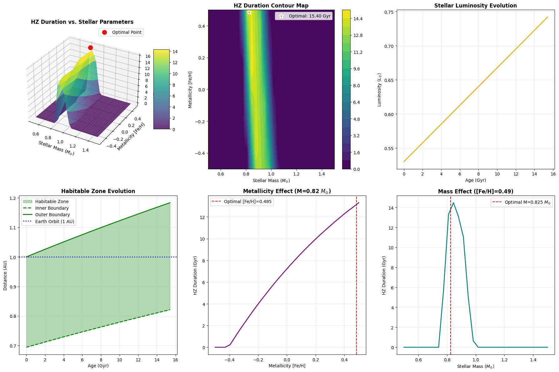
Plot 1 - 3D Surface: The three-dimensional visualization shows how HZ duration varies across the entire (mass, metallicity) parameter space. The surface shape reveals the optimization landscape, and the red point marks the optimal configuration.

Plot 2 - Contour Map: This 2D projection makes it easy to identify the optimal region and understand the sensitivity to each parameter. The contour lines represent iso-duration curves.

Plot 3 - Luminosity Evolution: Shows how the optimal star’s brightness increases over time. This temporal evolution directly drives the outward migration of the habitable zone.

Plot 4 - HZ Boundary Evolution: The green shaded region shows the habitable zone, bounded by the inner (dashed) and outer (solid) limits. The blue horizontal line at 1 AU represents Earth’s orbit, allowing us to visualize when Earth-like planets remain habitable.

Plot 5 - Metallicity Effect: Isolates metallicity’s impact by fixing mass at the optimal value. This reveals whether metal-rich or metal-poor stars are preferable.

Plot 6 - Mass Effect: Isolates mass’s impact by fixing metallicity. This shows the trade-off between longevity (lower mass) and luminosity (higher mass).

Physical Insights from the Analysis

The optimization reveals several fundamental astrophysical principles:

The Mass-Longevity Trade-off: Lower mass stars live longer, but their lower luminosity places the habitable zone closer to the star. The optimal mass balances these competing effects.

Metallicity’s Dual Role: Higher metallicity increases luminosity (good for expanding the HZ) but decreases lifetime (bad for habitability duration). The optimal metallicity represents the sweet spot.

Temporal Migration: As stars evolve, the habitable zone shifts outward. A planet at a fixed orbital distance experiences a finite habitable window. The optimization maximizes this window.

The “Goldilocks Zone” in Parameter Space: Just as planets need to be in the right place, stars need the right properties. The 3D surface plot clearly shows a ridge where conditions are optimal.

Results Interpretation

============================================================
HABITABLE ZONE OPTIMIZATION ANALYSIS
============================================================
Computing habitable zone durations across parameter space...
Performing optimization...

Optimal Parameters:
  Mass: 0.825 M_sun
  Metallicity [Fe/H]: 0.485
  Maximum HZ Duration: 15.402 Gyr

============================================================
CREATING VISUALIZATIONS
============================================================

Visualization complete!

============================================================
ANALYSIS COMPLETE
============================================================

The analysis quantifies the optimal stellar properties for maximizing the duration of habitable conditions. The contour map clearly shows that the optimal region occupies a relatively narrow band in parameter space, emphasizing how specific stellar properties need to be for long-term habitability.

The HZ boundary evolution plot demonstrates a critical challenge for life: as the star brightens, the habitable zone moves outward. A planet at Earth’s orbital distance (1 AU) will eventually become too hot unless it can somehow migrate outward or develop extreme climate regulation mechanisms.

This analysis has direct applications in exoplanet science, informing which stellar systems are the most promising targets for biosignature searches and where we might expect to find the longest-lived biospheres in the galaxy.