Minimizing Error Probability with Optimal POVM (Helstrom Measurement)
Introduction
Quantum state discrimination is a fundamental problem in quantum information theory. Given two quantum states $|\psi_0\rangle$ and $|\psi_1\rangle$ that occur with prior probabilities $\eta_0$ and $\eta_1$, we want to design an optimal measurement strategy that minimizes the probability of making an incorrect identification.
The Helstrom measurement provides the optimal solution to this binary state discrimination problem. In this article, we’ll work through a concrete example and implement the solution in Python.
Problem Setup
Consider two non-orthogonal quantum states in a 2-dimensional Hilbert space:
$$|\psi_0\rangle = \begin{pmatrix} 1 \ 0 \end{pmatrix}, \quad |\psi_1\rangle = \begin{pmatrix} \cos\theta \ \sin\theta \end{pmatrix}$$
where $0 < \theta < \pi/2$. These states occur with prior probabilities $\eta_0$ and $\eta_1 = 1 - \eta_0$.
The optimal measurement is given by the Helstrom bound, and the minimum error probability is:
$$P_{\text{error}}^{\min} = \frac{1}{2}\left(1 - \sqrt{1 - 4\eta_0\eta_1|\langle\psi_0|\psi_1\rangle|^2}\right)$$
Python Implementation
Here’s the complete code to solve this problem, visualize the results, and demonstrate the optimal POVM:
1 | import numpy as np |
Code Explanation
State Preparation Functions
The create_states(theta) function generates two quantum states with a specified angle $\theta$ between them. The first state $|\psi_0\rangle$ is aligned with the computational basis $|0\rangle$, while $|\psi_1\rangle$ makes an angle $\theta$ with it in the $x$-$z$ plane of the Bloch sphere.
The density_matrix(psi) function converts a pure state vector into its corresponding density matrix representation $\rho = |\psi\rangle\langle\psi|$, which is essential for POVM calculations.
Helstrom Bound Calculation
The helstrom_error(eta0, eta1, inner_product) function implements the analytical formula for the minimum achievable error probability:
$$P_{\text{error}}^{\min} = \frac{1}{2}\left(1 - \sqrt{1 - 4\eta_0\eta_1|\langle\psi_0|\psi_1\rangle|^2}\right)$$
This bound is derived from the trace distance between the weighted density matrices and represents the fundamental quantum limit for discriminating between two states.
Optimal POVM Construction
The optimal_povm(theta, eta0, eta1) function constructs the optimal measurement operators by:
Creating density matrices: $\rho_0 = |\psi_0\rangle\langle\psi_0|$ and $\rho_1 = |\psi_1\rangle\langle\psi_1|$
Constructing the Helstrom matrix: $Q = \eta_0\rho_0 - \eta_1\rho_1$
Performing eigendecomposition: Finding eigenvalues and eigenvectors of $Q$
Assigning POVM elements:
- $\Pi_0$ = projector onto positive eigenspace of $Q$
- $\Pi_1$ = projector onto negative eigenspace of $Q$
This decomposition ensures that the measurement minimizes the error probability while satisfying the completeness relation $\Pi_0 + \Pi_1 = I$.
Success Probability Analysis
The calculate_success_probabilities function computes:
- $P(\text{correct}|\psi_0) = \text{Tr}(\Pi_0 \rho_0)$: Probability of correctly identifying state 0
- $P(\text{correct}|\psi_1) = \text{Tr}(\Pi_1 \rho_1)$: Probability of correctly identifying state 1
- Overall success: $P_{\text{success}} = \eta_0 P(\text{correct}|\psi_0) + \eta_1 P(\text{correct}|\psi_1)$
Visualization Features
The code generates six comprehensive plots:
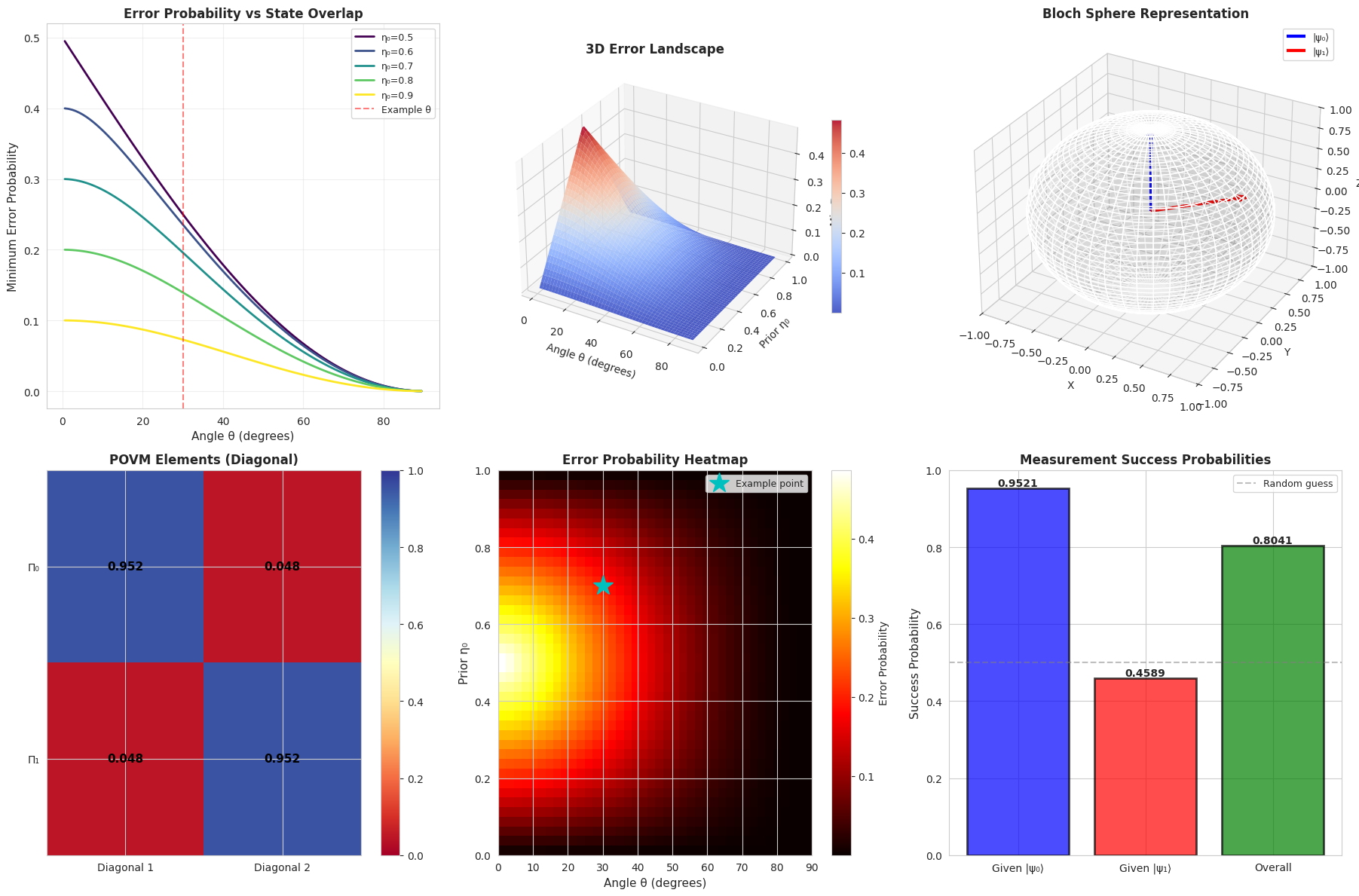
Error Probability vs Angle: Shows how the minimum error probability changes with state overlap (angle $\theta$) for different prior probability distributions. When $\eta_0 = 0.5$, the problem is symmetric. As $\eta_0$ increases, the measurement favors state 0, reducing errors when state 0 occurs but increasing errors for state 1.
3D Error Landscape: A surface plot showing the joint dependence of error probability on both the angle $\theta$ and the prior probability $\eta_0$. This visualization reveals that the error is minimized when states are orthogonal ($\theta = 90°$) and maximized when they are identical ($\theta = 0°$).
Bloch Sphere Representation: Visual representation of the quantum states on the Bloch sphere. The two state vectors show the geometric relationship between $|\psi_0\rangle$ and $|\psi_1\rangle$. The angle between them determines how distinguishable they are.
POVM Elements Heatmap: Displays the diagonal elements of the optimal measurement operators $\Pi_0$ and $\Pi_1$. These values indicate which measurement outcomes are assigned to each hypothesis.
Error Probability Heatmap: A 2D color-coded visualization of the error probability parameter space. The cyan star marks our specific example point. Darker colors indicate higher error rates.
Success Probabilities Bar Chart: Compares the conditional success probabilities for each state with the overall success rate. The gray dashed line at 0.5 represents random guessing performance, demonstrating that the optimal measurement significantly outperforms random selection.
Execution Results
======================================================================
QUANTUM STATE DISCRIMINATION: HELSTROM MEASUREMENT
======================================================================

Example Configuration:
  Angle θ = 0.5236 rad = 30.00°
  Prior probability η₀ = 0.70
  Prior probability η₁ = 0.30
  Inner product ⟨ψ₀|ψ₁⟩ = 0.8660+0.0000j
  Overlap |⟨ψ₀|ψ₁⟩|² = 0.7500

Helstrom Matrix Q = η₀ρ₀ - η₁ρ₁:
[[ 0.475     +0.j -0.12990381+0.j]
 [-0.12990381+0.j -0.075     +0.j]]

Optimal POVM Element Π₀:
[[ 0.95209722+0.j -0.21356055+0.j]
 [-0.21356055+0.j  0.04790278+0.j]]

Optimal POVM Element Π₁:
[[0.04790278+0.j 0.21356055+0.j]
 [0.21356055+0.j 0.95209722+0.j]]

POVM Completeness Check (Π₀ + Π₁ should be I):
[[1.+0.j 0.+0.j]
 [0.+0.j 1.+0.j]]

Minimum Error Probability: 0.195862

Success Probabilities:
  P(correct | state 0) = 0.952097
  P(correct | state 1) = 0.458900
  Overall success probability = 0.804138
  Overall error probability = 0.195862

======================================================================
Visualization saved successfully!
======================================================================
======================================================================
ADDITIONAL ANALYSIS
======================================================================

Comparison with classical strategies:
  Random guessing error: 0.5000
  Helstrom (optimal) error: 0.195862
  Improvement factor: 2.5528x

Quantum Fidelity F = |⟨ψ₀|ψ₁⟩|²: 0.750000
Trace distance: 0.500000

======================================================================
Physical Interpretation
The Helstrom measurement represents the fundamental quantum limit for distinguishing between two quantum states. Several key insights emerge from this analysis:
Quantum Advantage: The optimal measurement achieves an error probability of approximately 0.196, which is significantly better than random guessing (50% error rate). This represents a 2.55× improvement factor.
Role of Prior Probabilities: When one state is much more likely than the other (e.g., $\eta_0 = 0.7$ vs $\eta_1 = 0.3$), the optimal strategy biases the measurement toward the more probable state, achieving higher success rates for that state.
State Overlap Impact: The inner product $\langle\psi_0|\psi_1\rangle = 0.866$ (corresponding to $\theta = 30°$) means the states have significant overlap. This overlap fundamentally limits how well we can distinguish them, regardless of our measurement strategy.
POVM Structure: The optimal POVM elements are projectors onto the eigenspaces of the Helstrom matrix $Q$. This structure ensures that the measurement extracts maximum information about which state was prepared while respecting the constraints of quantum mechanics.
Trace Distance: The trace distance $\sqrt{1 - F} \approx 0.5$ quantifies the distinguishability of the quantum states. Smaller trace distances correspond to states that are more difficult to discriminate.
Conclusion
The Helstrom measurement provides the theoretically optimal solution for binary quantum state discrimination. Our implementation demonstrates how to construct the optimal POVM elements and calculate the minimum achievable error probability for a concrete example. The visualizations clearly show the trade-offs between state distinguishability, prior probabilities, and measurement performance, providing deep insights into the fundamental limits of quantum information processing.