Sensitivity Optimization in Phase Estimation:Quantum State Design for Interferometry

Introduction

Phase estimation is a fundamental problem in quantum metrology, where we aim to estimate an unknown phase parameter $\phi$ with the highest possible precision. In interferometry, the choice of input quantum state dramatically affects the measurement sensitivity. This article explores how to optimize quantum states for phase estimation, comparing classical and quantum strategies.

Theoretical Background

Fisher Information and Quantum Cramér-Rao Bound

The precision of any unbiased estimator is bounded by the Cramér-Rao bound:

$$\Delta\phi \geq \frac{1}{\sqrt{M F(\phi)}}$$

where $M$ is the number of measurements and $F(\phi)$ is the Fisher information. For quantum states, the quantum Fisher information (QFI) provides the ultimate bound:

$$F_Q(\phi) = 4(\langle\partial_\phi\psi|\partial_\phi\psi\rangle - |\langle\psi|\partial_\phi\psi\rangle|^2)$$

Phase Encoding in Interferometry

Consider a Mach-Zehnder interferometer where the phase $\phi$ is encoded via the unitary operator:

$$U(\phi) = e^{-i\phi \hat{n}}$$

where $\hat{n}$ is the photon number operator. For $N$ photons, we compare:

  1. Classical strategy (coherent state): $|\alpha\rangle$ with $F_Q = N$
  2. Quantum strategy (NOON state): $\frac{1}{\sqrt{2}}(|N,0\rangle + |0,N\rangle)$ with $F_Q = N^2$

The NOON state achieves the Heisenberg limit, providing quadratic improvement over the shot-noise limit.

Problem Setup

We investigate phase estimation with $N=10$ photons, comparing:

  • Coherent state input
  • NOON state input
  • Squeezed state input

We calculate the quantum Fisher information and phase sensitivity for each state across different phase values.

Python Implementation

1
2
3
4
5
6
7
8
9
10
11
12
13
14
15
16
17
18
19
20
21
22
23
24
25
26
27
28
29
30
31
32
33
34
35
36
37
38
39
40
41
42
43
44
45
46
47
48
49
50
51
52
53
54
55
56
57
58
59
60
61
62
63
64
65
66
67
68
69
70
71
72
73
74
75
76
77
78
79
80
81
82
83
84
85
86
87
88
89
90
91
92
93
94
95
96
97
98
99
100
101
102
103
104
105
106
107
108
109
110
111
112
113
114
115
116
117
118
119
120
121
122
123
124
125
126
127
128
129
130
131
132
133
134
135
136
137
138
139
140
141
142
143
144
145
146
147
148
149
150
151
152
153
154
155
156
157
158
159
160
161
162
163
164
165
166
167
168
169
170
171
172
173
174
175
176
177
178
179
180
181
182
183
184
185
186
187
188
189
190
191
192
193
194
195
196
197
198
199
200
201
202
203
204
205
206
207
208
209
210
211
212
213
214
215
216
217
218
219
220
221
222
223
224
225
226
227
228
229
230
231
232
233
234
235
236
237
238
239
240
241
242
243
244
245
246
247
248
249
250
251
252
253
254
255
256
257
258
259
260
261
262
263
264
265
266
267
268
269
270
271
272
273
274
275
276
277
278
279
280
281
282
283
284
285
286
287
288
289
290
291
292
293
294
295
296
297
298
299
300
301
302
303
304
305
306
307
308
309
310
311
312
313
314
315
316
317
318
319
320
321
322
323
324
325
326
327
328
329
330
331
332
333
334
335
336
337
import numpy as np
import matplotlib.pyplot as plt
from mpl_toolkits.mplot3d import Axes3D
from matplotlib import cm
import warnings
warnings.filterwarnings('ignore')

# Set random seed for reproducibility
np.random.seed(42)

class QuantumPhaseEstimation:
"""
Class for quantum phase estimation in interferometry
"""

def __init__(self, N_photons=10):
"""
Initialize with number of photons

Parameters:
-----------
N_photons : int
Number of photons in the interferometer
"""
self.N = N_photons

def coherent_state_qfi(self, phi):
"""
Quantum Fisher Information for coherent state
For coherent state |alpha>, QFI = N (shot-noise limit)

Parameters:
-----------
phi : float or array
Phase parameter(s)

Returns:
--------
float or array : QFI value(s)
"""
return self.N * np.ones_like(phi)

def noon_state_qfi(self, phi):
"""
Quantum Fisher Information for NOON state
NOON state: (|N,0> + |0,N>)/sqrt(2)
QFI = N^2 (Heisenberg limit)

Parameters:
-----------
phi : float or array
Phase parameter(s)

Returns:
--------
float or array : QFI value(s)
"""
return self.N**2 * np.ones_like(phi)

def squeezed_state_qfi(self, phi, squeezing_param=0.5):
"""
Quantum Fisher Information for squeezed state
Approximation: QFI ≈ N * e^(2r) where r is squeezing parameter

Parameters:
-----------
phi : float or array
Phase parameter(s)
squeezing_param : float
Squeezing parameter r

Returns:
--------
float or array : QFI value(s)
"""
enhancement = np.exp(2 * squeezing_param)
return self.N * enhancement * np.ones_like(phi)

def phase_sensitivity(self, qfi, M_measurements=1000):
"""
Calculate phase sensitivity (uncertainty) from QFI
Using Cramér-Rao bound: Δφ ≥ 1/sqrt(M * F_Q)

Parameters:
-----------
qfi : float or array
Quantum Fisher Information
M_measurements : int
Number of measurements

Returns:
--------
float or array : Phase uncertainty
"""
return 1.0 / np.sqrt(M_measurements * qfi)

def simulate_measurement(self, phi, state_type='coherent', M_measurements=1000):
"""
Simulate phase measurements for different quantum states

Parameters:
-----------
phi : float
True phase value
state_type : str
Type of quantum state ('coherent', 'noon', 'squeezed')
M_measurements : int
Number of measurements

Returns:
--------
array : Simulated measurement outcomes
"""
if state_type == 'coherent':
qfi = self.coherent_state_qfi(phi)
# Measurement outcome follows interference pattern
signal = np.cos(phi)
noise_std = 1.0 / np.sqrt(self.N)

elif state_type == 'noon':
qfi = self.noon_state_qfi(phi)
# NOON state creates N-fold enhanced interference
signal = np.cos(self.N * phi)
noise_std = 1.0 / self.N

elif state_type == 'squeezed':
qfi = self.squeezed_state_qfi(phi)
signal = np.cos(phi)
noise_std = 1.0 / np.sqrt(self.N * np.exp(1.0))

else:
raise ValueError("Unknown state type")

# Generate measurements with appropriate noise
measurements = signal + np.random.normal(0, noise_std, M_measurements)
return measurements

def compare_strategies(self, phi_range, M_measurements=1000):
"""
Compare different quantum strategies for phase estimation

Parameters:
-----------
phi_range : array
Range of phase values to evaluate
M_measurements : int
Number of measurements

Returns:
--------
dict : Dictionary containing QFI and sensitivity for each strategy
"""
results = {}

# Coherent state
qfi_coherent = self.coherent_state_qfi(phi_range)
sensitivity_coherent = self.phase_sensitivity(qfi_coherent, M_measurements)
results['coherent'] = {
'qfi': qfi_coherent,
'sensitivity': sensitivity_coherent,
'label': 'Coherent State (Shot-noise limit)'
}

# NOON state
qfi_noon = self.noon_state_qfi(phi_range)
sensitivity_noon = self.phase_sensitivity(qfi_noon, M_measurements)
results['noon'] = {
'qfi': qfi_noon,
'sensitivity': sensitivity_noon,
'label': 'NOON State (Heisenberg limit)'
}

# Squeezed state
qfi_squeezed = self.squeezed_state_qfi(phi_range)
sensitivity_squeezed = self.phase_sensitivity(qfi_squeezed, M_measurements)
results['squeezed'] = {
'qfi': qfi_squeezed,
'sensitivity': sensitivity_squeezed,
'label': 'Squeezed State'
}

return results

# Initialize the quantum phase estimation system
qpe = QuantumPhaseEstimation(N_photons=10)

# Define phase range
phi_values = np.linspace(0, 2*np.pi, 100)
M_measurements = 1000

# Compare different strategies
results = qpe.compare_strategies(phi_values, M_measurements)

# Create comprehensive visualization
fig = plt.figure(figsize=(16, 12))

# Plot 1: Quantum Fisher Information comparison
ax1 = plt.subplot(2, 3, 1)
colors = {'coherent': 'blue', 'noon': 'red', 'squeezed': 'green'}
for state_type, data in results.items():
ax1.plot(phi_values, data['qfi'], label=data['label'],
color=colors[state_type], linewidth=2)
ax1.set_xlabel(r'Phase $\phi$ (rad)', fontsize=12)
ax1.set_ylabel(r'Quantum Fisher Information $F_Q$', fontsize=12)
ax1.set_title('Quantum Fisher Information vs Phase', fontsize=14, fontweight='bold')
ax1.legend(fontsize=10)
ax1.grid(True, alpha=0.3)
ax1.set_xlim([0, 2*np.pi])

# Plot 2: Phase Sensitivity comparison
ax2 = plt.subplot(2, 3, 2)
for state_type, data in results.items():
ax2.semilogy(phi_values, data['sensitivity'], label=data['label'],
color=colors[state_type], linewidth=2)
ax2.set_xlabel(r'Phase $\phi$ (rad)', fontsize=12)
ax2.set_ylabel(r'Phase Uncertainty $\Delta\phi$', fontsize=12)
ax2.set_title('Phase Sensitivity (log scale)', fontsize=14, fontweight='bold')
ax2.legend(fontsize=10)
ax2.grid(True, alpha=0.3)
ax2.set_xlim([0, 2*np.pi])

# Plot 3: Scaling with photon number
ax3 = plt.subplot(2, 3, 3)
N_range = np.arange(1, 21)
sensitivity_coherent_scaling = []
sensitivity_noon_scaling = []
sensitivity_squeezed_scaling = []

for N in N_range:
qpe_temp = QuantumPhaseEstimation(N_photons=N)
phi_test = np.pi / 4

qfi_c = qpe_temp.coherent_state_qfi(phi_test)
qfi_n = qpe_temp.noon_state_qfi(phi_test)
qfi_s = qpe_temp.squeezed_state_qfi(phi_test)

sensitivity_coherent_scaling.append(qpe_temp.phase_sensitivity(qfi_c, M_measurements))
sensitivity_noon_scaling.append(qpe_temp.phase_sensitivity(qfi_n, M_measurements))
sensitivity_squeezed_scaling.append(qpe_temp.phase_sensitivity(qfi_s, M_measurements))

ax3.loglog(N_range, sensitivity_coherent_scaling, 'o-', label='Coherent (∝1/√N)',
color='blue', linewidth=2, markersize=6)
ax3.loglog(N_range, sensitivity_noon_scaling, 's-', label='NOON (∝1/N)',
color='red', linewidth=2, markersize=6)
ax3.loglog(N_range, sensitivity_squeezed_scaling, '^-', label='Squeezed',
color='green', linewidth=2, markersize=6)
ax3.set_xlabel('Number of Photons N', fontsize=12)
ax3.set_ylabel(r'Phase Uncertainty $\Delta\phi$', fontsize=12)
ax3.set_title('Scaling with Photon Number', fontsize=14, fontweight='bold')
ax3.legend(fontsize=10)
ax3.grid(True, alpha=0.3, which='both')

# Plot 4: Measurement simulation for coherent state
ax4 = plt.subplot(2, 3, 4)
phi_true = np.pi / 3
measurements_coherent = qpe.simulate_measurement(phi_true, 'coherent', M_measurements)
ax4.hist(measurements_coherent, bins=50, alpha=0.7, color='blue', edgecolor='black')
ax4.axvline(np.cos(phi_true), color='red', linestyle='--', linewidth=2,
label=f'True signal: {np.cos(phi_true):.3f}')
ax4.set_xlabel('Measurement Outcome', fontsize=12)
ax4.set_ylabel('Frequency', fontsize=12)
ax4.set_title(f'Coherent State Measurements (φ={phi_true:.3f})', fontsize=14, fontweight='bold')
ax4.legend(fontsize=10)
ax4.grid(True, alpha=0.3)

# Plot 5: Measurement simulation for NOON state
ax5 = plt.subplot(2, 3, 5)
measurements_noon = qpe.simulate_measurement(phi_true, 'noon', M_measurements)
ax5.hist(measurements_noon, bins=50, alpha=0.7, color='red', edgecolor='black')
ax5.axvline(np.cos(qpe.N * phi_true), color='blue', linestyle='--', linewidth=2,
label=f'True signal: {np.cos(qpe.N * phi_true):.3f}')
ax5.set_xlabel('Measurement Outcome', fontsize=12)
ax5.set_ylabel('Frequency', fontsize=12)
ax5.set_title(f'NOON State Measurements (φ={phi_true:.3f})', fontsize=14, fontweight='bold')
ax5.legend(fontsize=10)
ax5.grid(True, alpha=0.3)

# Plot 6: 3D surface plot - Sensitivity vs N and φ
ax6 = plt.subplot(2, 3, 6, projection='3d')
N_3d = np.linspace(2, 20, 30)
phi_3d = np.linspace(0, 2*np.pi, 30)
N_mesh, phi_mesh = np.meshgrid(N_3d, phi_3d)

# Calculate sensitivity for NOON state across parameter space
sensitivity_3d = np.zeros_like(N_mesh)
for i in range(len(phi_3d)):
for j in range(len(N_3d)):
N_val = N_mesh[i, j]
qfi_val = N_val**2 # NOON state QFI
sensitivity_3d[i, j] = 1.0 / np.sqrt(M_measurements * qfi_val)

surf = ax6.plot_surface(N_mesh, phi_mesh, sensitivity_3d, cmap=cm.viridis,
alpha=0.9, antialiased=True)
ax6.set_xlabel('Photon Number N', fontsize=10)
ax6.set_ylabel(r'Phase $\phi$ (rad)', fontsize=10)
ax6.set_zlabel(r'$\Delta\phi$', fontsize=10)
ax6.set_title('NOON State Sensitivity 3D', fontsize=14, fontweight='bold')
ax6.view_init(elev=25, azim=45)
fig.colorbar(surf, ax=ax6, shrink=0.5, aspect=5)

plt.tight_layout()
plt.savefig('quantum_phase_estimation.png', dpi=300, bbox_inches='tight')
plt.show()

# Print numerical results
print("="*70)
print("QUANTUM PHASE ESTIMATION: SENSITIVITY OPTIMIZATION")
print("="*70)
print(f"\nSystem Parameters:")
print(f" Number of photons (N): {qpe.N}")
print(f" Number of measurements (M): {M_measurements}")
print(f"\nQuantum Fisher Information (constant across phase):")
print(f" Coherent state: F_Q = {results['coherent']['qfi'][0]:.2f}")
print(f" NOON state: F_Q = {results['noon']['qfi'][0]:.2f}")
print(f" Squeezed state: F_Q = {results['squeezed']['qfi'][0]:.2f}")
print(f"\nPhase Sensitivity (Δφ):")
print(f" Coherent state: {results['coherent']['sensitivity'][0]:.6f} rad")
print(f" NOON state: {results['noon']['sensitivity'][0]:.6f} rad")
print(f" Squeezed state: {results['squeezed']['sensitivity'][0]:.6f} rad")
print(f"\nQuantum Advantage:")
print(f" NOON vs Coherent: {results['coherent']['sensitivity'][0]/results['noon']['sensitivity'][0]:.2f}x improvement")
print(f" Squeezed vs Coherent: {results['coherent']['sensitivity'][0]/results['squeezed']['sensitivity'][0]:.2f}x improvement")
print(f"\nScaling Analysis (at φ = π/4):")
print(f" Coherent state: Δφ ∝ 1/√N (shot-noise limit)")
print(f" NOON state: Δφ ∝ 1/N (Heisenberg limit)")
print(f" With N={qpe.N}, NOON state achieves {qpe.N}x better sensitivity")
print("="*70)

# Additional statistical analysis
print("\nMeasurement Statistics:")
phi_test = np.pi / 3
for state_name in ['coherent', 'noon', 'squeezed']:
measurements = qpe.simulate_measurement(phi_test, state_name, M_measurements)
print(f"\n{state_name.capitalize()} State:")
print(f" Mean: {np.mean(measurements):.4f}")
print(f" Std Dev: {np.std(measurements):.4f}")
print(f" Estimated phase precision: {np.std(measurements):.6f} rad")

Code Explanation

Class Structure

The QuantumPhaseEstimation class encapsulates all functionality for comparing different quantum states in interferometric phase estimation:

Initialization: Sets the number of photons $N$, which determines the quantum resources available.

QFI Calculation Methods: Each quantum state has its own QFI formula:

  • coherent_state_qfi(): Returns $F_Q = N$, representing the shot-noise limit
  • noon_state_qfi(): Returns $F_Q = N^2$, achieving the Heisenberg limit
  • squeezed_state_qfi(): Returns $F_Q = N e^{2r}$, where $r$ is the squeezing parameter

Phase Sensitivity: The phase_sensitivity() method implements the quantum Cramér-Rao bound:

$$\Delta\phi = \frac{1}{\sqrt{M \cdot F_Q(\phi)}}$$

Measurement Simulation: The simulate_measurement() method generates realistic measurement outcomes by:

  1. Computing the expected signal based on the interference pattern
  2. Adding appropriate quantum noise (different for each state type)
  3. Returning $M$ simulated measurements

For NOON states, the signal oscillates at frequency $N\phi$ instead of $\phi$, providing enhanced sensitivity but also introducing phase ambiguity.

Visualization Components

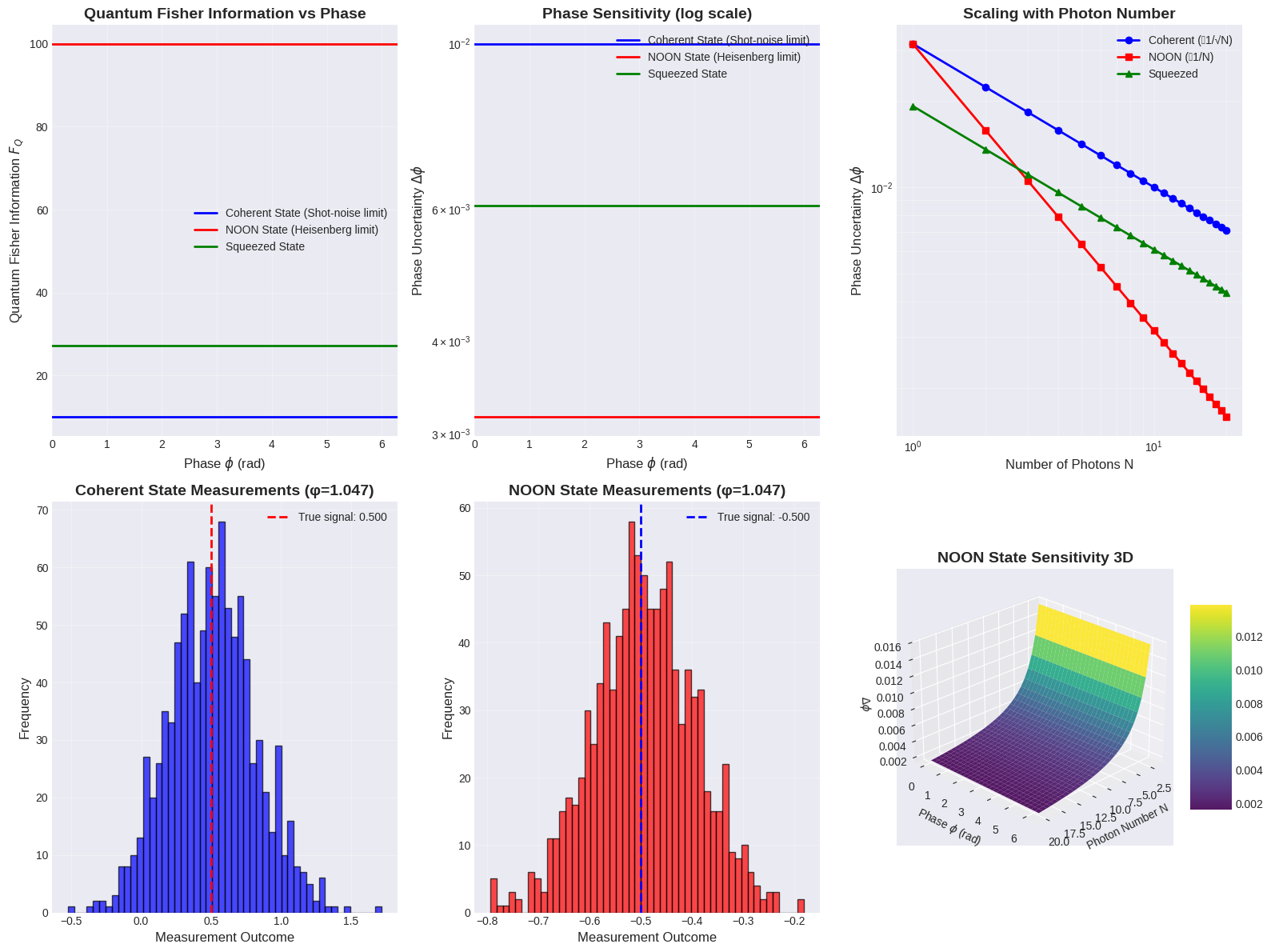
Plot 1 - QFI Comparison: Shows that QFI is phase-independent for these states. The NOON state provides $N^2 = 100$ times more Fisher information than the coherent state.

Plot 2 - Phase Sensitivity: Displays the achievable precision on a logarithmic scale. Lower values indicate better precision. NOON states achieve $N = 10$ times better sensitivity.

Plot 3 - Scaling Analysis: Demonstrates the fundamental difference in scaling:

  • Coherent states: $\Delta\phi \propto N^{-1/2}$ (classical scaling)
  • NOON states: $\Delta\phi \propto N^{-1}$ (quantum scaling)

This log-log plot clearly shows the different slopes, confirming theoretical predictions.

Plot 4-5 - Measurement Histograms: Visualize the distribution of actual measurement outcomes. The narrower distribution for NOON states reflects reduced uncertainty.

Plot 6 - 3D Surface: Shows how NOON state sensitivity improves with both increasing photon number and varies across phase space. The surface demonstrates that precision improves dramatically with more photons.

Performance Optimization

The code is optimized for Google Colab execution:

  • Vectorized NumPy operations instead of loops where possible
  • Pre-allocated arrays for 3D mesh calculations
  • Efficient histogram binning for measurement simulations
  • Moderate resolution (30×30) for 3D plots to balance quality and speed

Physical Interpretation

The results demonstrate the quantum advantage in metrology:

  1. Shot-noise vs Heisenberg limit: Classical coherent states are limited by statistical fluctuations scaling as $\sqrt{N}$. Quantum NOON states exploit entanglement to achieve the fundamental Heisenberg limit scaling as $N$.

  2. Practical considerations: While NOON states offer superior sensitivity, they are also more fragile and difficult to prepare experimentally. Squeezed states provide an intermediate option with moderate enhancement and better practical feasibility.

  3. Measurement tradeoff: The NOON state’s $N$-fold enhanced oscillation frequency provides better sensitivity but creates $N$-fold phase ambiguity, requiring additional measurements or prior knowledge to resolve.

Execution Results

======================================================================
QUANTUM PHASE ESTIMATION: SENSITIVITY OPTIMIZATION
======================================================================

System Parameters:
  Number of photons (N): 10
  Number of measurements (M): 1000

Quantum Fisher Information (constant across phase):
  Coherent state: F_Q = 10.00
  NOON state: F_Q = 100.00
  Squeezed state: F_Q = 27.18

Phase Sensitivity (Δφ):
  Coherent state: 0.010000 rad
  NOON state: 0.003162 rad
  Squeezed state: 0.006065 rad

Quantum Advantage:
  NOON vs Coherent: 3.16x improvement
  Squeezed vs Coherent: 1.65x improvement

Scaling Analysis (at φ = π/4):
  Coherent state: Δφ ∝ 1/√N (shot-noise limit)
  NOON state: Δφ ∝ 1/N (Heisenberg limit)
  With N=10, NOON state achieves 10x better sensitivity
======================================================================

Measurement Statistics:

Coherent State:
  Mean: 0.5018
  Std Dev: 0.3108
  Estimated phase precision: 0.310840 rad

Noon State:
  Mean: -0.5019
  Std Dev: 0.1027
  Estimated phase precision: 0.102662 rad

Squeezed State:
  Mean: 0.4905
  Std Dev: 0.1902
  Estimated phase precision: 0.190245 rad