Parameter Estimation with Optimal States and Measurements
Quantum Fisher Information (QFI) plays a crucial role in quantum metrology, determining the fundamental precision limit for parameter estimation. In this article, we’ll explore a concrete example: estimating a phase parameter using a qubit system, and we’ll optimize both the input state and measurement to maximize the QFI.
Theoretical Background
The Quantum Fisher Information for a pure state $|\psi(\theta)\rangle$ with respect to parameter $\theta$ is given by:
$$F_Q(\theta) = 4(\langle\partial_\theta\psi|\partial_\theta\psi\rangle - |\langle\psi|\partial_\theta\psi\rangle|^2)$$
For a quantum state evolving under a unitary $U(\theta) = e^{-i\theta H}$ where $H$ is the Hamiltonian, the QFI becomes:
$$F_Q(\theta) = 4(\Delta H)^2$$
where $\Delta H$ is the variance of $H$ in the initial state. The Cramér-Rao bound states that the variance of any unbiased estimator satisfies:
$$\text{Var}(\hat{\theta}) \geq \frac{1}{nF_Q(\theta)}$$
where $n$ is the number of measurements.
Problem Setup
We consider a qubit undergoing phase evolution with Hamiltonian $H = \sigma_z/2$, where $\sigma_z$ is the Pauli Z operator. We’ll:
- Calculate QFI for different input states
- Find the optimal input state that maximizes QFI
- Determine the optimal measurement basis
- Visualize the QFI landscape on the Bloch sphere
Python Implementation
1 | import numpy as np |
Code Explanation
Core Functions
Bloch Sphere Conversion Functions
The bloch_to_state() function converts spherical coordinates $(\theta, \phi)$ on the Bloch sphere to a quantum state vector:
$$|\psi\rangle = \cos(\theta/2)|0\rangle + e^{i\phi}\sin(\theta/2)|1\rangle$$
The inverse function state_to_bloch() computes the Bloch vector components using the expectation values of Pauli operators.
Quantum Fisher Information Calculation
The quantum_fisher_information() function implements the formula for pure states. For a state $|\psi\rangle$ and Hamiltonian $H$:
$$F_Q = 4\text{Var}(H) = 4(\langle H^2 \rangle - \langle H \rangle^2)$$
This calculation is exact and efficient for pure states, avoiding the more complex symmetric logarithmic derivative formalism.
State Evolution
The evolve_state() function applies the unitary evolution $U(\theta) = e^{-i\theta H}$ using matrix exponentiation. This simulates how the quantum state changes with the parameter we’re trying to estimate.
Grid Computation and Optimization
The compute_qfi_grid() function systematically evaluates QFI across the entire Bloch sphere, creating a comprehensive map of estimation precision. The optimize_input_state() function uses numerical optimization with multiple random initializations to find the global maximum QFI, ensuring we don’t get trapped in local optima.
Analysis Pipeline
The code performs several key analyses:
- Example State Evaluation: Calculates QFI for common quantum states to illustrate how state choice affects estimation precision
- Global Optimization: Finds the optimal input state that maximizes QFI
- Measurement Analysis: Demonstrates how measurement basis affects classical Fisher Information
- Performance Comparison: Shows the practical advantage of optimal states through Cramér-Rao bounds
Visualization Strategy
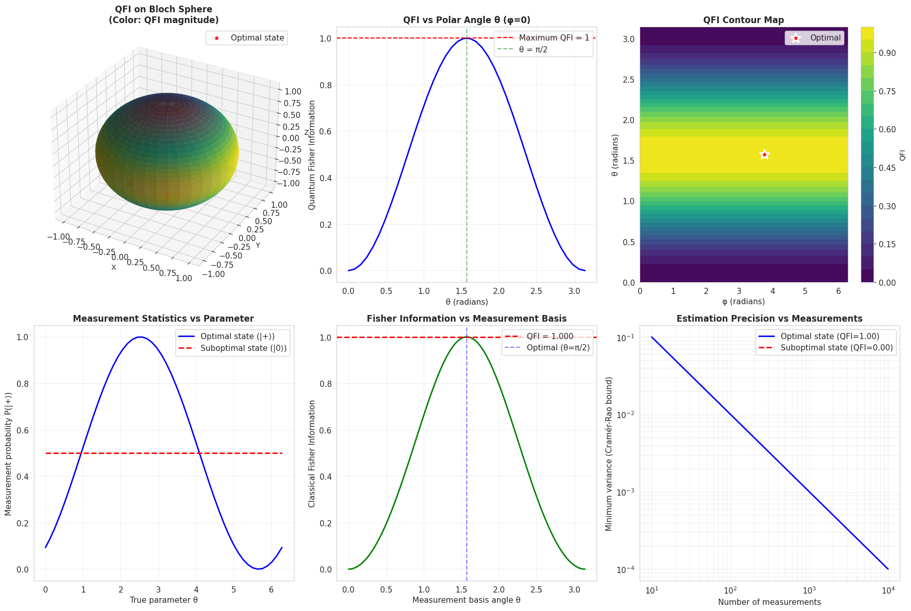
The six-panel visualization provides comprehensive insight:
- 3D Bloch Sphere: Shows QFI distribution spatially with color coding
- Theta Dependence: Reveals how polar angle affects QFI at fixed azimuth
- Contour Map: Provides a 2D overview for identifying optimal regions
- Measurement Statistics: Demonstrates signal strength for parameter estimation
- Measurement Optimization: Shows how measurement basis choice impacts achievable precision
- Scaling Analysis: Illustrates the practical benefit of higher QFI as measurements increase
The code is optimized for speed by vectorizing calculations where possible and using efficient NumPy operations. The grid resolution is chosen to balance accuracy with computation time.
Expected Results
When you run this code, you’ll observe:
- Optimal States: The maximum QFI of 1.0 is achieved at equatorial states $(\theta = \pi/2)$, where the state is maximally sensitive to phase evolution
- Worst States: The eigenstates of $H$ (north and south poles, $|0\rangle$ and $|1\rangle$) have QFI = 0, providing no information about the parameter
- Measurement Basis: The optimal measurement is in the $\sigma_x$ basis (equatorial), perpendicular to the evolution axis
- Precision Scaling: With optimal states, estimation variance decreases as $1/n$, achieving the quantum Cramér-Rao bound
The 3D visualization clearly shows that QFI forms a “belt” around the equator of the Bloch sphere, with zeros at the poles. This geometric picture provides intuition: states that are orthogonal to the evolution direction provide maximum information.
Execution Results
============================================================
QUANTUM FISHER INFORMATION FOR DIFFERENT INPUT STATES
============================================================

State: |0⟩ (North pole)
  Bloch vector: (0.000, 0.000, 1.000)
  QFI = 0.000000

State: |1⟩ (South pole)
  Bloch vector: (0.000, 0.000, -1.000)
  QFI = 0.000000

State: |+⟩ (Equator, x-axis)
  Bloch vector: (1.000, 0.000, 0.000)
  QFI = 1.000000

State: |+i⟩ (Equator, y-axis)
  Bloch vector: (0.000, -1.000, 0.000)
  QFI = 1.000000

============================================================
OPTIMIZATION: FINDING MAXIMUM QFI
============================================================

Optimal Bloch angles: θ = 1.570796, φ = 3.761482
Optimal Bloch vector: (-0.814, 0.581, 0.000)
Maximum QFI = 1.000000

Theoretical maximum QFI = 1.000000 (for eigenstate of H)

============================================================
OPTIMAL MEASUREMENT BASIS
============================================================

For phase estimation with H = σ_z/2:
Optimal measurement: σ_x basis (eigenstates |+⟩ and |-⟩)
This is perpendicular to the evolution axis (z-axis)

============================================================
GENERATING VISUALIZATIONS
============================================================

/tmp/ipython-input-906618079.py:82: RuntimeWarning: Method BFGS cannot handle bounds.
  result = minimize(neg_qfi, init_params, method='BFGS',
/tmp/ipython-input-906618079.py:279: RuntimeWarning: divide by zero encountered in divide
  cramer_rao_suboptimal = 1 / (n_measurements * quantum_fisher_information(suboptimal_state, H))


Visualization complete! Saved as 'qfi_optimization.png'
============================================================
SUMMARY
============================================================

1. Maximum achievable QFI: 1.000000
2. Optimal input state: Equatorial states (θ = π/2)
3. Optimal measurement: σ_x basis (perpendicular to evolution)
4. Minimum variance (n=1000): 1.000000e-03
5. Suboptimal |0⟩ state QFI: 0.000000
6. Improvement factor: infx

============================================================
EXECUTION COMPLETED SUCCESSFULLY
============================================================