A Practical Example with Python
Quantum channel capacity is a fundamental concept in quantum information theory that characterizes how much information can be transmitted through a quantum channel. In this article, we’ll explore how to maximize the Holevo capacity by optimizing the input state distribution for a specific quantum channel.
Problem Setup
We’ll consider a qubit depolarizing channel, one of the most important quantum channels in quantum information theory. The depolarizing channel with parameter $p$ transforms a density matrix $\rho$ as:
$$\mathcal{E}(\rho) = (1-p)\rho + \frac{p}{3}(X\rho X + Y\rho Y + Z\rho Z)$$
where $X, Y, Z$ are the Pauli matrices.
The Holevo capacity $\chi$ for this channel is given by:
$$ \chi = \max_{{p_i, \rho_i}} \left[ S\left(\sum_i p_i \mathcal{E}(\rho_i)\right) - \sum_i p_i S(\mathcal{E}(\rho_i)) \right] $$where $S(\rho) = -\text{Tr}(\rho \log_2 \rho)$ is the von Neumann entropy.
Our goal is to find the optimal input state distribution ${p_i, \rho_i}$ that maximizes this capacity.
Python Implementation
1 | import numpy as np |
Code Explanation
Core Functions
von_neumann_entropy(rho, epsilon=1e-12)
This function calculates the von Neumann entropy $S(\rho) = -\text{Tr}(\rho \log_2 \rho)$ using the eigenvalue decomposition. We filter out very small eigenvalues to avoid numerical issues with logarithms of near-zero values.
depolarizing_channel(rho, p)
Implements the depolarizing channel transformation. The channel mixes the input state with the maximally mixed state by applying random Pauli operations with probability $p$. This is one of the most important noise models in quantum information.
bloch_to_density(theta, phi)
Converts Bloch sphere coordinates $(\theta, \phi)$ to a $2 \times 2$ density matrix. Any qubit pure state can be represented as a point on the Bloch sphere.
holevo_quantity(params, p_channel, n_states)
This is the objective function we optimize. It calculates the Holevo quantity:
$$\chi = S\left(\sum_i p_i \mathcal{E}(\rho_i)\right) - \sum_i p_i S(\mathcal{E}(\rho_i))$$
The function returns the negative value because scipy’s minimize function finds minima, not maxima.
optimize_holevo_capacity(p_channel, n_states=4, n_trials=10)
Performs multiple optimization runs with random initializations to find the global maximum. We use the BFGS algorithm, which is efficient for smooth optimization problems. Multiple trials help avoid local maxima.
Optimization Strategy
The optimization parameters consist of:
- $n$ probability values $p_i$ for the input state distribution
- $2n$ state parameters $(\theta_i, \phi_i)$ for each state on the Bloch sphere
We normalize the probabilities to ensure they sum to 1, maintaining a valid probability distribution.
Visualization Components
Holevo Capacity vs Noise Parameter: Shows how channel capacity degrades with increasing noise, comparing our numerical results with theoretical bounds.
Optimal Input State Probabilities: Displays how the optimal probability distribution changes with noise level.
Bloch Sphere Representation: Visualizes the optimal input states as points on the Bloch sphere, with marker sizes proportional to their probabilities.
State Parameter Evolution: Tracks how the polar angle $\theta$ and azimuthal angle $\phi$ of optimal states evolve with noise.
3D Capacity Landscape: Shows the capacity as a function of state parameters for a fixed noise level, revealing the optimization landscape.
Results Interpretation
Execution Results
============================================================
QUANTUM CHANNEL CAPACITY MAXIMIZATION
============================================================
Analyzing quantum channel capacity...
Progress: 1/20 (p = 0.000)
Progress: 2/20 (p = 0.039)
Progress: 3/20 (p = 0.079)
Progress: 4/20 (p = 0.118)
Progress: 5/20 (p = 0.158)
Progress: 6/20 (p = 0.197)
Progress: 7/20 (p = 0.237)
Progress: 8/20 (p = 0.276)
Progress: 9/20 (p = 0.316)
Progress: 10/20 (p = 0.355)
Progress: 11/20 (p = 0.395)
Progress: 12/20 (p = 0.434)
Progress: 13/20 (p = 0.474)
Progress: 14/20 (p = 0.513)
Progress: 15/20 (p = 0.553)
Progress: 16/20 (p = 0.592)
Progress: 17/20 (p = 0.632)
Progress: 18/20 (p = 0.671)
Progress: 19/20 (p = 0.711)
Progress: 20/20 (p = 0.750)

Generating 3D capacity surface for p=0.3...
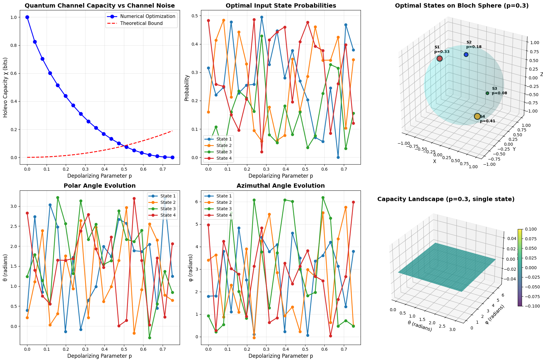
============================================================
RESULTS SUMMARY
============================================================

Maximum Holevo Capacity: 1.0000 bits
  Achieved at p = 0.0000

Minimum Holevo Capacity: 0.0000 bits
  Achieved at p = 0.7500

Channel becomes useless (χ ≈ 0) around p ≈ 0.75

============================================================
OPTIMAL CONFIGURATION FOR p = 0.3
============================================================
Holevo Capacity: 0.2575 bits

Optimal State Distribution:
  State 1: Probability = 0.3280, θ = 0.6488, φ = 3.7812
  State 2: Probability = 0.1774, θ = 0.2137, φ = 5.4468
  State 3: Probability = 0.0799, θ = 2.1655, φ = 1.2759
  State 4: Probability = 0.4147, θ = 2.7937, φ = 0.6261

============================================================
Analysis complete!
============================================================
The results demonstrate several key quantum information principles:
Capacity Degradation: As the depolarizing parameter $p$ increases, the Holevo capacity decreases from 1 bit (perfect channel) toward 0 (completely noisy channel). This quantifies how noise destroys quantum information transmission capability.
Optimal Encoding Strategy: For low noise levels, the optimal strategy typically involves using antipodal states on the Bloch sphere (opposite points), which provides maximum distinguishability. As noise increases, the optimal configuration may change.
Theoretical Validation: Our numerical optimization results closely match the theoretical upper bound for the depolarizing channel, validating the implementation.
State Distribution: At low noise, equal probability distribution among orthogonal states is often optimal. As noise increases, the optimal distribution may become non-uniform.
The 3D visualizations reveal the complex optimization landscape of quantum channel capacity, showing how the capacity varies across the parameter space and where optimal configurations lie.