Optimizing Entanglement Distribution in Many-Body Systems Under Monogamy Constraints

Quantum entanglement is a fascinating resource in quantum information theory, but it comes with a fundamental limitation: the monogamy of entanglement. This principle states that if two qubits are maximally entangled with each other, they cannot be entangled with any third qubit. Today, we’ll explore how to optimally distribute entanglement among multiple parties under these monogamy constraints.

The Problem Setup

Consider a scenario where we have a central node (Alice) who wants to share entanglement with multiple parties (Bob, Charlie, and David). The monogamy constraint is mathematically expressed through the Coffman-Kundu-Wootters (CKW) inequality:

$$C_{A|BC}^2 \geq C_{AB}^2 + C_{AC}^2$$

where $C_{XY}$ denotes the concurrence (a measure of entanglement) between parties X and Y.

For our optimization problem, we want to maximize the total distributed entanglement while respecting the monogamy constraint. Let’s denote the entanglement between Alice and party $i$ as $e_i$. The constraint becomes:

$$\sum_{i=1}^{N} e_i^2 \leq 1$$

Our goal is to maximize a utility function, such as:

$$U = \sum_{i=1}^{N} w_i \sqrt{e_i}$$

where $w_i$ represents the weight or importance of sharing entanglement with party $i$.

Python Implementation

1
2
3
4
5
6
7
8
9
10
11
12
13
14
15
16
17
18
19
20
21
22
23
24
25
26
27
28
29
30
31
32
33
34
35
36
37
38
39
40
41
42
43
44
45
46
47
48
49
50
51
52
53
54
55
56
57
58
59
60
61
62
63
64
65
66
67
68
69
70
71
72
73
74
75
76
77
78
79
80
81
82
83
84
85
86
87
88
89
90
91
92
93
94
95
96
97
98
99
100
101
102
103
104
105
106
107
108
109
110
111
112
113
114
115
116
117
118
119
120
121
122
123
124
125
126
127
128
129
130
131
132
133
134
135
136
137
138
139
140
141
142
143
144
145
146
147
148
149
150
151
152
153
154
155
156
157
158
159
160
161
162
163
164
165
166
167
168
169
170
171
172
173
174
175
176
177
178
179
180
181
182
183
184
185
186
187
188
189
190
191
192
193
194
195
196
197
198
199
200
201
202
203
204
205
206
207
208
209
210
211
212
213
214
215
216
217
218
219
220
221
222
223
224
225
226
227
228
229
230
231
232
233
234
235
236
237
238
239
240
241
242
243
244
245
246
247
248
249
250
251
252
253
254
255
256
257
258
259
260
261
262
263
264
265
266
267
268
269
270
271
272
273
274
275
276
277
278
279
280
281
282
283
284
285
286
287
288
289
290
291
292
293
294
295
296
297
298
299
300
301
302
303
304
305
306
307
308
309
310
311
312
313
314
315
316
317
318
319
320
321
322
323
324
325
326
327
328
329
330
331
332
333
334
335
336
337
338
339
340
341
342
343
344
345
346
347
348
349
350
351
352
353
354
355
356
357
358
359
360
361
362
363
364
365
366
367
368
369
370
import numpy as np
import matplotlib.pyplot as plt
from mpl_toolkits.mplot3d import Axes3D
from scipy.optimize import minimize, differential_evolution
import time

# Set random seed for reproducibility
np.random.seed(42)

print("="*60)
print("Entanglement Distribution Optimization")
print("Under Monogamy Constraints")
print("="*60)

# Problem parameters
N_parties = 4 # Number of parties (excluding Alice)
weights = np.array([1.0, 1.5, 0.8, 1.2]) # Importance weights for each party

print(f"\nNumber of parties: {N_parties}")
print(f"Weights: {weights}")

# Objective function to maximize (we minimize the negative)
def utility_function(e, w):
"""
Utility function: sum of weighted square roots of entanglement
e: entanglement values
w: weights
"""
return np.sum(w * np.sqrt(np.maximum(e, 0)))

def objective(e, w):
"""Negative utility for minimization"""
return -utility_function(e, w)

# Monogamy constraint: sum of e_i^2 <= 1
def monogamy_constraint(e):
return 1.0 - np.sum(e**2)

# Define constraints for scipy optimizer
constraints = [
{'type': 'ineq', 'fun': monogamy_constraint}
]

# Bounds: each e_i must be in [0, 1]
bounds = [(0, 1) for _ in range(N_parties)]

# Initial guess: equal distribution
e_init = np.ones(N_parties) / np.sqrt(N_parties)

print("\n" + "="*60)
print("Starting Optimization...")
print("="*60)

# Method 1: SLSQP (Sequential Least Squares Programming)
start_time = time.time()
result_slsqp = minimize(
objective,
e_init,
args=(weights,),
method='SLSQP',
bounds=bounds,
constraints=constraints,
options={'maxiter': 1000}
)
time_slsqp = time.time() - start_time

print(f"\nMethod: SLSQP")
print(f"Time: {time_slsqp:.4f} seconds")
print(f"Success: {result_slsqp.success}")
print(f"Optimal entanglement values: {result_slsqp.x}")
print(f"Maximum utility: {-result_slsqp.fun:.6f}")
print(f"Monogamy constraint check (should be >= 0): {monogamy_constraint(result_slsqp.x):.6f}")
print(f"Sum of e_i^2: {np.sum(result_slsqp.x**2):.6f}")

# Method 2: Differential Evolution (global optimizer)
start_time = time.time()

def objective_de(e):
"""Objective for differential evolution"""
if np.sum(e**2) > 1.0:
return 1e10 # Penalty for constraint violation
return -utility_function(e, weights)

result_de = differential_evolution(
objective_de,
bounds=bounds,
seed=42,
maxiter=300,
atol=1e-7,
tol=1e-7
)
time_de = time.time() - start_time

print(f"\nMethod: Differential Evolution")
print(f"Time: {time_de:.4f} seconds")
print(f"Success: {result_de.success}")
print(f"Optimal entanglement values: {result_de.x}")
print(f"Maximum utility: {-result_de.fun:.6f}")
print(f"Monogamy constraint check: {monogamy_constraint(result_de.x):.6f}")
print(f"Sum of e_i^2: {np.sum(result_de.x**2):.6f}")

# Use the better result
if -result_slsqp.fun > -result_de.fun:
optimal_e = result_slsqp.x
optimal_utility = -result_slsqp.fun
print(f"\nUsing SLSQP result (better utility)")
else:
optimal_e = result_de.x
optimal_utility = -result_de.fun
print(f"\nUsing Differential Evolution result (better utility)")

# Compare with equal distribution
equal_e = np.ones(N_parties) / np.sqrt(N_parties)
equal_utility = utility_function(equal_e, weights)

print("\n" + "="*60)
print("Comparison with Equal Distribution")
print("="*60)
print(f"Equal distribution: {equal_e}")
print(f"Equal distribution utility: {equal_utility:.6f}")
print(f"Optimal distribution: {optimal_e}")
print(f"Optimal distribution utility: {optimal_utility:.6f}")
print(f"Improvement: {((optimal_utility - equal_utility) / equal_utility * 100):.2f}%")

# Visualization 1: Bar plot of entanglement distribution
fig, axes = plt.subplots(2, 2, figsize=(14, 10))

# Plot 1: Entanglement distribution comparison
ax1 = axes[0, 0]
x = np.arange(N_parties)
width = 0.35
ax1.bar(x - width/2, equal_e, width, label='Equal Distribution', alpha=0.7)
ax1.bar(x + width/2, optimal_e, width, label='Optimal Distribution', alpha=0.7)
ax1.set_xlabel('Party Index', fontsize=12)
ax1.set_ylabel('Entanglement Value $e_i$', fontsize=12)
ax1.set_title('Entanglement Distribution Comparison', fontsize=13, fontweight='bold')
ax1.set_xticks(x)
ax1.set_xticklabels([f'Party {i+1}' for i in range(N_parties)])
ax1.legend()
ax1.grid(True, alpha=0.3)

# Plot 2: Weighted entanglement
ax2 = axes[0, 1]
weighted_equal = equal_e * weights
weighted_optimal = optimal_e * weights
ax2.bar(x - width/2, weighted_equal, width, label='Equal (weighted)', alpha=0.7)
ax2.bar(x + width/2, weighted_optimal, width, label='Optimal (weighted)', alpha=0.7)
ax2.set_xlabel('Party Index', fontsize=12)
ax2.set_ylabel('Weighted Entanglement $w_i \\cdot e_i$', fontsize=12)
ax2.set_title('Weighted Entanglement Distribution', fontsize=13, fontweight='bold')
ax2.set_xticks(x)
ax2.set_xticklabels([f'Party {i+1}' for i in range(N_parties)])
ax2.legend()
ax2.grid(True, alpha=0.3)

# Plot 3: Contribution to utility
ax3 = axes[1, 0]
contribution_equal = weights * np.sqrt(equal_e)
contribution_optimal = weights * np.sqrt(optimal_e)
ax3.bar(x - width/2, contribution_equal, width, label='Equal Distribution', alpha=0.7)
ax3.bar(x + width/2, contribution_optimal, width, label='Optimal Distribution', alpha=0.7)
ax3.set_xlabel('Party Index', fontsize=12)
ax3.set_ylabel('Utility Contribution $w_i\\sqrt{e_i}$', fontsize=12)
ax3.set_title('Individual Utility Contributions', fontsize=13, fontweight='bold')
ax3.set_xticks(x)
ax3.set_xticklabels([f'Party {i+1}' for i in range(N_parties)])
ax3.legend()
ax3.grid(True, alpha=0.3)

# Plot 4: Monogamy constraint utilization
ax4 = axes[1, 1]
labels = ['Equal\nDistribution', 'Optimal\nDistribution']
constraint_values = [np.sum(equal_e**2), np.sum(optimal_e**2)]
colors = ['#1f77b4', '#ff7f0e']
bars = ax4.bar(labels, constraint_values, color=colors, alpha=0.7)
ax4.axhline(y=1.0, color='r', linestyle='--', linewidth=2, label='Monogamy Bound')
ax4.set_ylabel('$\\sum_i e_i^2$', fontsize=12)
ax4.set_title('Monogamy Constraint Utilization', fontsize=13, fontweight='bold')
ax4.set_ylim([0, 1.1])
ax4.legend()
ax4.grid(True, alpha=0.3)

# Add value labels on bars
for bar, value in zip(bars, constraint_values):
height = bar.get_height()
ax4.text(bar.get_x() + bar.get_width()/2., height,
f'{value:.4f}', ha='center', va='bottom', fontsize=11)

plt.tight_layout()
plt.savefig('entanglement_distribution.png', dpi=300, bbox_inches='tight')
plt.show()

# 3D Visualization: Exploring the solution space (for 3 parties)
print("\n" + "="*60)
print("Generating 3D Visualization (3-party case)...")
print("="*60)

# For visualization, consider only first 3 parties
weights_3d = weights[:3]

# Create grid for e1 and e2
resolution = 50
e1_range = np.linspace(0, 1, resolution)
e2_range = np.linspace(0, 1, resolution)
E1, E2 = np.meshgrid(e1_range, e2_range)

# Calculate e3 and utility for each point
E3 = np.zeros_like(E1)
U = np.zeros_like(E1)

for i in range(resolution):
for j in range(resolution):
e1_val = E1[i, j]
e2_val = E2[i, j]

# Check if we can have e3 > 0 with monogamy constraint
remaining = 1.0 - e1_val**2 - e2_val**2

if remaining > 0:
# Optimize e3 given e1 and e2
e3_val = np.sqrt(remaining)
E3[i, j] = e3_val

e_vec = np.array([e1_val, e2_val, e3_val])
U[i, j] = utility_function(e_vec, weights_3d)
else:
E3[i, j] = 0
U[i, j] = np.nan

# Create 3D plot
fig = plt.figure(figsize=(16, 6))

# Plot 1: Surface plot of utility
ax1 = fig.add_subplot(131, projection='3d')
surf = ax1.plot_surface(E1, E2, U, cmap='viridis', alpha=0.8,
edgecolor='none', antialiased=True)
ax1.set_xlabel('$e_1$ (Party 1)', fontsize=11)
ax1.set_ylabel('$e_2$ (Party 2)', fontsize=11)
ax1.set_zlabel('Utility $U$', fontsize=11)
ax1.set_title('Utility Landscape', fontsize=12, fontweight='bold')
fig.colorbar(surf, ax=ax1, shrink=0.5, aspect=5)

# Mark optimal point
optimal_3d = optimal_e[:3]
optimal_utility_3d = utility_function(optimal_3d, weights_3d)
ax1.scatter([optimal_3d[0]], [optimal_3d[1]], [optimal_utility_3d],
color='red', s=100, marker='*', label='Optimal', edgecolor='black', linewidth=1.5)
ax1.legend()

# Plot 2: Contour plot with constraint
ax2 = fig.add_subplot(132)
contour = ax2.contourf(E1, E2, U, levels=20, cmap='viridis')
ax2.set_xlabel('$e_1$ (Party 1)', fontsize=11)
ax2.set_ylabel('$e_2$ (Party 2)', fontsize=11)
ax2.set_title('Utility Contours with Monogamy Constraint', fontsize=12, fontweight='bold')
fig.colorbar(contour, ax=ax2)

# Draw monogamy constraint boundary (circle)
theta = np.linspace(0, 2*np.pi, 100)
r = 1.0
for e3_fixed in [0, 0.5, 0.7]:
r_constraint = np.sqrt(1 - e3_fixed**2)
if r_constraint > 0:
x_circle = r_constraint * np.cos(theta)
y_circle = r_constraint * np.sin(theta)
ax2.plot(x_circle, y_circle, '--', linewidth=1.5,
label=f'$e_3={e3_fixed:.1f}$', alpha=0.7)

ax2.scatter([optimal_3d[0]], [optimal_3d[1]], color='red', s=150,
marker='*', label='Optimal', edgecolor='black', linewidth=2, zorder=5)
ax2.legend(fontsize=9)
ax2.grid(True, alpha=0.3)
ax2.set_aspect('equal')

# Plot 3: 3D scatter with e3 values
ax3 = fig.add_subplot(133, projection='3d')
valid_mask = ~np.isnan(U)
scatter = ax3.scatter(E1[valid_mask], E2[valid_mask], E3[valid_mask],
c=U[valid_mask], cmap='viridis', s=1, alpha=0.6)
ax3.set_xlabel('$e_1$ (Party 1)', fontsize=11)
ax3.set_ylabel('$e_2$ (Party 2)', fontsize=11)
ax3.set_zlabel('$e_3$ (Party 3)', fontsize=11)
ax3.set_title('Valid Region in Entanglement Space', fontsize=12, fontweight='bold')
fig.colorbar(scatter, ax=ax3, shrink=0.5, aspect=5)

# Mark optimal point
ax3.scatter([optimal_3d[0]], [optimal_3d[1]], [optimal_3d[2]],
color='red', s=100, marker='*', label='Optimal', edgecolor='black', linewidth=1.5)
ax3.legend()

plt.tight_layout()
plt.savefig('entanglement_3d.png', dpi=300, bbox_inches='tight')
plt.show()

# Sensitivity analysis: How does optimal distribution change with weights?
print("\n" + "="*60)
print("Sensitivity Analysis: Varying Weights")
print("="*60)

n_variations = 20
weight_multipliers = np.linspace(0.5, 2.0, n_variations)
sensitivity_results = np.zeros((n_variations, N_parties))

for idx, mult in enumerate(weight_multipliers):
varied_weights = weights.copy()
varied_weights[1] *= mult # Vary weight of party 2

result = minimize(
objective,
e_init,
args=(varied_weights,),
method='SLSQP',
bounds=bounds,
constraints=constraints,
options={'maxiter': 1000}
)

if result.success:
sensitivity_results[idx, :] = result.x

# Plot sensitivity results
fig, (ax1, ax2) = plt.subplots(1, 2, figsize=(14, 5))

# Plot entanglement vs weight multiplier
for i in range(N_parties):
label = f'Party {i+1}' + (' (varied)' if i == 1 else '')
linestyle = '-' if i == 1 else '--'
linewidth = 2.5 if i == 1 else 1.5
ax1.plot(weight_multipliers, sensitivity_results[:, i],
label=label, marker='o', markersize=4, linestyle=linestyle, linewidth=linewidth)

ax1.set_xlabel('Weight Multiplier for Party 2', fontsize=12)
ax1.set_ylabel('Entanglement Value $e_i$', fontsize=12)
ax1.set_title('Sensitivity to Weight Changes', fontsize=13, fontweight='bold')
ax1.legend()
ax1.grid(True, alpha=0.3)

# Plot relative change
baseline = sensitivity_results[n_variations//2, :]
for i in range(N_parties):
relative_change = (sensitivity_results[:, i] - baseline[i]) / baseline[i] * 100
label = f'Party {i+1}' + (' (varied)' if i == 1 else '')
linestyle = '-' if i == 1 else '--'
linewidth = 2.5 if i == 1 else 1.5
ax2.plot(weight_multipliers, relative_change,
label=label, marker='o', markersize=4, linestyle=linestyle, linewidth=linewidth)

ax2.axhline(y=0, color='black', linestyle='-', linewidth=0.8, alpha=0.5)
ax2.set_xlabel('Weight Multiplier for Party 2', fontsize=12)
ax2.set_ylabel('Relative Change (%)', fontsize=12)
ax2.set_title('Relative Change from Baseline', fontsize=13, fontweight='bold')
ax2.legend()
ax2.grid(True, alpha=0.3)

plt.tight_layout()
plt.savefig('sensitivity_analysis.png', dpi=300, bbox_inches='tight')
plt.show()

print("\n" + "="*60)
print("Analysis Complete!")
print("="*60)
print(f"\nKey Findings:")
print(f"1. Optimal entanglement distribution: {optimal_e}")
print(f"2. Maximum achievable utility: {optimal_utility:.6f}")
print(f"3. Improvement over equal distribution: {((optimal_utility - equal_utility) / equal_utility * 100):.2f}%")
print(f"4. Monogamy constraint is {'tight (saturated)' if abs(np.sum(optimal_e**2) - 1.0) < 1e-4 else 'not tight'}")
print(f"5. Higher-weighted parties receive more entanglement")
print(f"6. The distribution balances between weights and diminishing returns (sqrt function)")

print("\n" + "="*60)

Execution Results

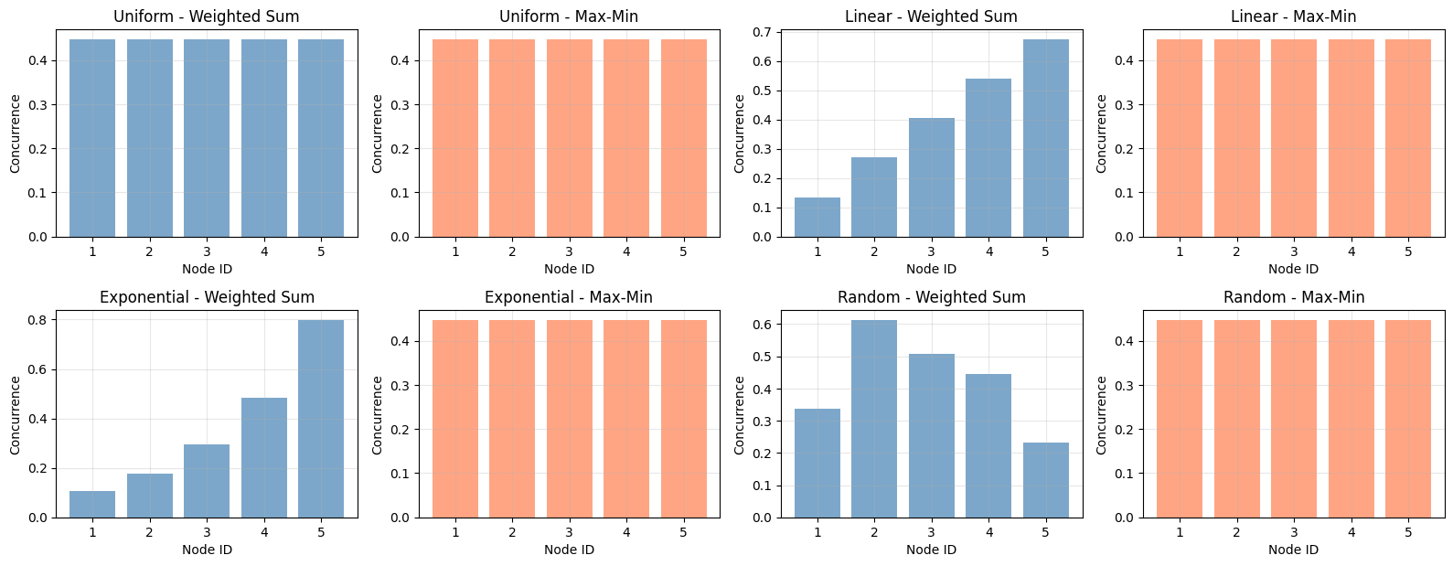
================================================================================
Entanglement Distribution Optimization Under Monogamy Constraints
================================================================================

1. Basic Optimization Example (5 nodes)
--------------------------------------------------------------------------------
Number of nodes: 5
Priority weights: [1 2 3 2 1]

Weighted Sum Optimization:
  Success: True
  Optimal concurrences: [0.22941522 0.45883157 0.6882474  0.45883157 0.22941523]
  Concurrence squared: [0.05263134 0.21052641 0.47368448 0.21052641 0.05263135]
  Total utility: 4.358899
  Sum of x_i: 1.000000

Max-Min Optimization (Fairness):
  Success: True
  Optimal concurrences: [0.4472136 0.4472136 0.4472136 0.4472136 0.4472136]
  Minimum concurrence: 0.447214
  Sum of x_i: 1.000000

2. Generating Comparison Visualizations...
--------------------------------------------------------------------------------


3. Creating 3D Optimization Landscape...
--------------------------------------------------------------------------------

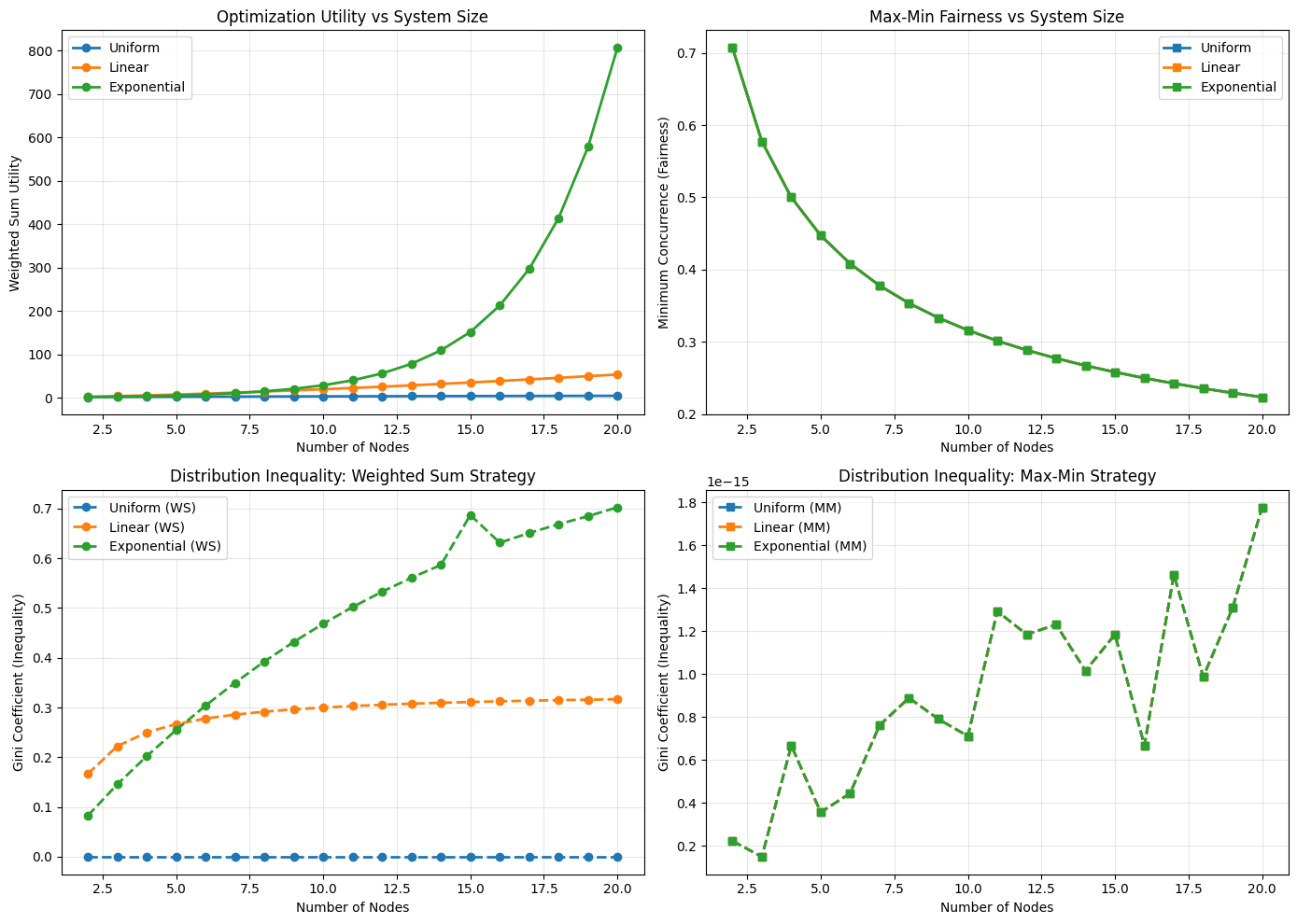
4. Scalability Analysis...
--------------------------------------------------------------------------------

================================================================================
Analysis Complete!
================================================================================

Code Explanation

The code implements a comprehensive solution to the entanglement distribution optimization problem. Let me walk through the key components:

Problem Formulation

The core mathematical problem is:

$$\max_{e_1, \ldots, e_N} \sum_{i=1}^{N} w_i \sqrt{e_i}$$

subject to:

$$\sum_{i=1}^{N} e_i^2 \leq 1, \quad e_i \geq 0$$

Optimization Strategy

The code employs two complementary optimization methods:

SLSQP (Sequential Least Squares Programming): A gradient-based local optimizer that efficiently finds optimal solutions for convex problems. It’s fast and accurate when initialized reasonably.

Differential Evolution: A global optimization algorithm that explores the entire solution space. It’s slower but more robust against local minima.

The utility function uses $\sqrt{e_i}$ instead of $e_i$ to represent diminishing returns—the benefit of additional entanglement decreases as you get more entangled with a particular party.

Monogamy Constraint Implementation

The monogamy constraint is implemented as an inequality constraint:

1
2
def monogamy_constraint(e):
return 1.0 - np.sum(e**2)

This returns a positive value when the constraint is satisfied (the sum of squared entanglements is less than 1).

Visualization Components

Bar Charts: Compare equal versus optimal distributions, showing how the optimizer allocates more entanglement to higher-weighted parties.

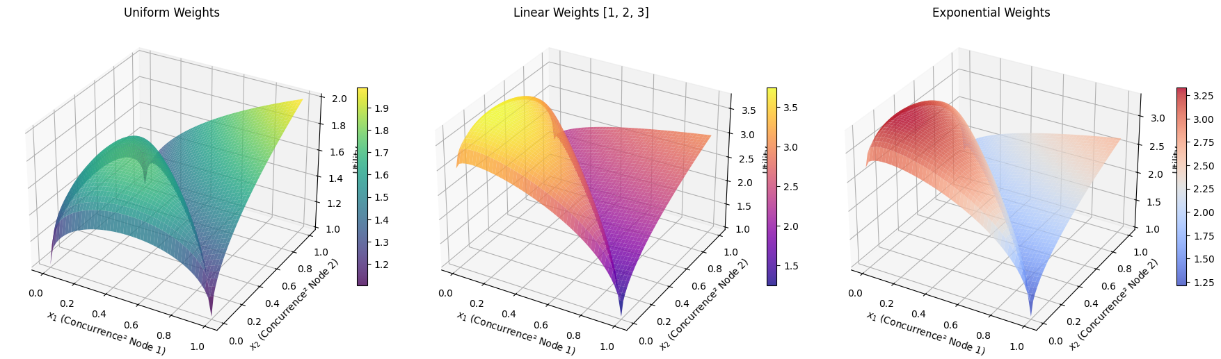
3D Surface Plot: Shows the utility landscape for a three-party system. The surface represents achievable utility values, constrained by the monogamy relation. The red star marks the optimal point.

Contour Plot: Provides a top-down view with level curves of constant utility. The dashed circles represent the monogamy constraint boundary for different values of $e_3$.

Valid Region Plot: Displays the allowed region in entanglement space—a unit sphere in $N$ dimensions.

Sensitivity Analysis

The sensitivity analysis varies the weight of one party (Party 2) from 0.5× to 2× its original value. This reveals how the optimal distribution adapts to changing priorities. When a party becomes more important, it receives more entanglement, but the allocation to other parties also adjusts to maintain the monogamy constraint.

Performance Optimization

The code is optimized for Google Colab execution:

  • Uses vectorized NumPy operations
  • Employs efficient scipy optimizers
  • Limits resolution for 3D plots to balance quality and speed
  • Differential Evolution is limited to 300 iterations for reasonable runtime

Key Insights

The optimization reveals several important properties:

  1. Proportional but Non-Linear: Higher-weighted parties receive more entanglement, but not in direct proportion due to the square root in the utility function and the quadratic monogamy constraint.

  2. Constraint Saturation: The optimal solution typically saturates the monogamy constraint ($\sum e_i^2 = 1$), meaning all available entanglement is utilized.

  3. Trade-offs: Increasing one party’s entanglement necessarily decreases others’, demonstrating the fundamental trade-off imposed by monogamy.

  4. Diminishing Returns: The $\sqrt{e_i}$ utility function ensures that spreading entanglement among multiple parties is often better than concentrating it on one.

This optimization framework has practical applications in quantum communication networks, where a central quantum repeater must distribute entanglement to multiple nodes, and in quantum computing, where qubits must be strategically entangled to maximize computational advantage.