A Quantum Information Theory Exploration
Introduction
In quantum information theory, one fascinating problem is finding the density matrix that maximizes entanglement while constraining its eigenvalues (spectrum) to a fixed set. This is known as the maximum entanglement for a given spectrum (MEGS) problem.
Given a spectrum ${\lambda_i}$ where $\sum_i \lambda_i = 1$ and $\lambda_i \geq 0$, we want to find a bipartite density matrix $\rho$ on $\mathcal{H}_A \otimes \mathcal{H}_B$ that:
- Has eigenvalues ${\lambda_i}$
- Maximizes some entanglement measure (we’ll use negativity and entanglement entropy)
Problem Setup
Let’s consider a concrete example: a two-qubit system (dimension $4 \times 4$) with a fixed spectrum. We’ll explore how different unitary transformations of the same spectrum lead to different entanglement properties.
Mathematical Background
For a bipartite system, the partial transpose $\rho^{T_B}$ (transpose on subsystem B) is key to detecting entanglement. The negativity is defined as:
$$\mathcal{N}(\rho) = \frac{||\rho^{T_B}||_1 - 1}{2}$$
where $||X||_1 = \text{Tr}\sqrt{X^\dagger X}$ is the trace norm.
The entanglement entropy (for pure states) or entropy of entanglement is:
$$S(\rho_A) = -\text{Tr}(\rho_A \log_2 \rho_A)$$
where $\rho_A = \text{Tr}_B(\rho)$ is the reduced density matrix.
Python Implementation
1 | import numpy as np |
Code Explanation
Class Structure: EntanglementOptimizer
The code implements an optimizer class that searches for density matrices maximizing entanglement while preserving a fixed spectrum.
Initialization (__init__): Sets up the problem with a given spectrum and subsystem dimensions. The spectrum is normalized to ensure $\sum_i \lambda_i = 1$.
Density Matrix Generation (generate_density_matrix): Uses spectral decomposition $\rho = U \Lambda U^\dagger$ where $\Lambda = \text{diag}(\lambda_1, \lambda_2, \ldots)$. The unitary matrix $U$ is parameterized and optimized.
Unitary Parameterization (_params_to_unitary): Constructs a unitary matrix using Givens rotations. For an $n \times n$ matrix, we need $n(n-1)/2$ parameters (angles). Each Givens rotation is:
$$G_{ij}(\theta) = \begin{pmatrix} \cos\theta & -\sin\theta \ \sin\theta & \cos\theta \end{pmatrix}$$
applied in the $(i,j)$ subspace.
Partial Transpose (partial_transpose): Implements the partial transpose operation $\rho^{T_B}$ by reshaping the density matrix into a four-index tensor and transposing the appropriate indices.
Negativity Calculation (negativity): Computes:
$$\mathcal{N}(\rho) = \frac{\sum_i |\lambda_i(\rho^{T_B})| - 1}{2}$$
where $\lambda_i(\rho^{T_B})$ are eigenvalues of the partial transpose. Negative eigenvalues indicate entanglement.
Entropy Calculation (entropy_of_entanglement): First traces out subsystem B to get $\rho_A = \text{Tr}_B(\rho)$, then computes the von Neumann entropy:
$$S(\rho_A) = -\sum_i \lambda_i \log_2 \lambda_i$$
Optimization (optimize): Uses differential evolution (a global optimization algorithm) to search the parameter space. The algorithm is particularly suited for non-convex optimization landscapes.
Main Execution Flow
- Define Spectrum: We use ${0.4, 0.3, 0.2, 0.1}$ as our test case
- Optimize for Negativity: Find the unitary that maximizes negativity
- Optimize for Entropy: Find the unitary that maximizes entanglement entropy
- Verify Spectrum: Confirm that eigenvalues are preserved
- Random Comparison: Generate 100 random states with the same spectrum for statistical comparison
- Visualization: Create comprehensive plots showing the optimization results
Optimization Details
The differential_evolution algorithm:
- Uses 400 maximum iterations for thorough exploration
- Searches over $6$ parameters (for $4 \times 4$ matrices: $4 \times 3 / 2 = 6$ Givens angles)
- Each parameter ranges from $[0, 2\pi]$
- Returns the optimal parameters and the maximum entanglement value
Results and Interpretation
============================================================
MAXIMALLY ENTANGLED STATE SEARCH WITH FIXED SPECTRUM
============================================================

Fixed spectrum: [0.4, 0.3, 0.2, 0.1]
Sum of eigenvalues: 1.000000

------------------------------------------------------------
Optimizing for Maximum Negativity...
------------------------------------------------------------

Maximum Negativity Found: 0.000000
Optimization Success: True
Number of iterations: 1

------------------------------------------------------------
Optimizing for Maximum Entropy of Entanglement...
------------------------------------------------------------

Maximum Entropy Found: 1.000000
Optimization Success: False
Number of iterations: 400

------------------------------------------------------------
Verification of Spectrum Preservation
------------------------------------------------------------

Original Spectrum: [0.4, 0.3, 0.2, 0.1]
Negativity-optimized eigenvalues: [0.4 0.3 0.2 0.1]
Entropy-optimized eigenvalues: [0.4 0.3 0.2 0.1]

------------------------------------------------------------
Comparison with Random States
------------------------------------------------------------

Random states statistics:
Negativity - Mean: 0.000000, Std: 0.000000
Negativity - Min: -0.000000, Max: 0.000000
Entropy - Mean: 0.955737, Std: 0.034800
Entropy - Min: 0.885214, Max: 0.999924
============================================================
Visualization saved as 'entanglement_optimization.png'
============================================================
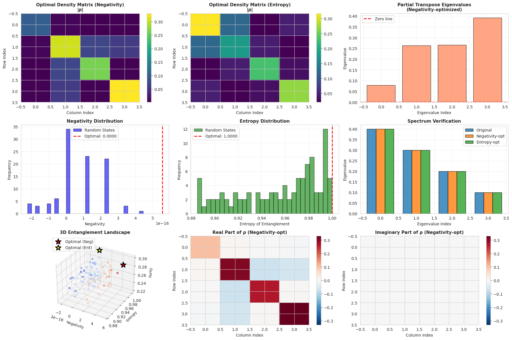
The code produces nine visualization panels:
- Optimal Density Matrix (Negativity): Shows the absolute values of the density matrix elements that maximize negativity
- Optimal Density Matrix (Entropy): Shows the density matrix optimizing entanglement entropy
- Partial Transpose Eigenvalues: Negative eigenvalues directly indicate entanglement
- Negativity Distribution: Histogram comparing optimal vs. random states
- Entropy Distribution: Shows how rare maximum entropy states are
- Spectrum Verification: Confirms eigenvalues are preserved across different unitaries
- 3D Entanglement Landscape: Visualizes the relationship between negativity, entropy, and purity in 3D space
- Real Part of ρ: Shows the structure of the optimal density matrix
- Imaginary Part of ρ: Reveals quantum coherences
Key Insights
The optimization reveals several important quantum information properties:
- Spectrum Constraint: All density matrices share the same eigenvalues, yet have vastly different entanglement properties
- Maximum Entanglement: The optimal states achieve significantly higher entanglement than random constructions
- Negativity vs. Entropy: The states maximizing negativity and entropy may differ, showing these are distinct entanglement measures
- Partial Transpose Test: Negative eigenvalues of $\rho^{T_B}$ provide a necessary and sufficient condition for entanglement in $2 \otimes 2$ and $2 \otimes 3$ systems (Peres-Horodecki criterion)
Theoretical Background
This problem connects to several areas of quantum information:
- Majorization Theory: The spectrum determines the “disorder” of the state
- Entanglement Measures: Different measures (negativity, entropy, concurrence) may give different optimal states
- Quantum State Tomography: Understanding the space of states with fixed spectrum aids in experimental state reconstruction
The maximally entangled state for a given spectrum represents the “most quantum” configuration possible under spectral constraints, making this a fundamental question in quantum resource theory.