Optimizing Drug Molecular Design

Balancing Efficacy, Side Effects, and Solubility

Introduction

Drug discovery is a complex optimization problem where we need to balance multiple competing objectives: maximizing therapeutic efficacy (binding affinity to target), minimizing side effects (off-target binding), and ensuring adequate solubility for bioavailability. In this blog post, I’ll walk through a concrete example using multi-objective optimization techniques in Python.

Problem Formulation

We’ll design a hypothetical small molecule drug by optimizing its molecular descriptors. Our objectives are:

1. Maximize binding affinity to the target protein (lower binding energy is better)
2. Minimize off-target binding (reduce side effects)
3. Optimize solubility (LogP should be in the ideal range)

Mathematical Model

We’ll use the following simplified models:

Binding Affinity (to be minimized):

$$E_{\text{binding}} = -10 \exp\left(-0.1(x_1 - 5)^2\right) - 8 \exp\left(-0.05(x_2 - 3)^2\right) + 0.5x_3$$

Off-target Binding (to be minimized):

$$E_{\text{off-target}} = 5 \exp\left(-0.08(x_1 - 7)^2\right) + 3x_2^{0.5}$$

Solubility LogP (target range: 2-3):

$$\text{LogP} = 0.5x_1 + 0.3x_2 - 0.2x_3$$

$$\text{Solubility Penalty} = |\text{LogP} - 2.5|$$

Where:

• $x_1$: Molecular weight proxy (normalized, 0-10)
• $x_2$: Hydrophobicity index (0-10)
• $x_3$: Hydrogen bond donors/acceptors (0-10)

Python Implementation

import numpy as np
import matplotlib.pyplot as plt
from scipy.optimize import differential_evolution, minimize
from mpl_toolkits.mplot3d import Axes3D
import seaborn as sns

# Set random seed for reproducibility
np.random.seed(42)

# Define objective functions
def binding_affinity(x):
    """
    Target binding affinity (lower is better - stronger binding)
    x[0]: Molecular weight proxy (0-10)
    x[1]: Hydrophobicity index (0-10)
    x[2]: H-bond donors/acceptors (0-10)
    """
    return -10 * np.exp(-0.1 * (x[0] - 5)**2) - 8 * np.exp(-0.05 * (x[1] - 3)**2) + 0.5 * x[2]

def off_target_binding(x):
    """
    Off-target binding (lower is better - fewer side effects)
    """
    return 5 * np.exp(-0.08 * (x[0] - 7)**2) + 3 * np.sqrt(x[1] + 0.1)

def solubility_penalty(x):
    """
    Solubility represented by LogP
    Ideal range: 2-3 (for oral bioavailability)
    Penalty increases as we deviate from ideal range
    """
    logP = 0.5 * x[0] + 0.3 * x[1] - 0.2 * x[2]
    target_logP = 2.5
    return np.abs(logP - target_logP)

def combined_objective(x, weights):
    """
    Weighted sum of all objectives
    weights: [w_affinity, w_offtarget, w_solubility]
    """
    affinity = binding_affinity(x)
    offtarget = off_target_binding(x)
    solubility = solubility_penalty(x)
    
    # Normalize objectives (approximate ranges)
    affinity_norm = (affinity + 18) / 10  # Range roughly -18 to -8
    offtarget_norm = offtarget / 10  # Range roughly 0 to 10
    solubility_norm = solubility / 3  # Range roughly 0 to 3
    
    return weights[0] * affinity_norm + weights[1] * offtarget_norm + weights[2] * solubility_norm

# Optimization using Differential Evolution
bounds = [(0, 10), (0, 10), (0, 10)]

# Different weight scenarios
scenarios = {
    'Balanced': [1.0, 1.0, 1.0],
    'Efficacy-focused': [2.0, 0.5, 0.5],
    'Safety-focused': [0.5, 2.0, 1.0],
    'Solubility-focused': [0.5, 0.5, 2.0]
}

results = {}
print("="*70)
print("DRUG MOLECULAR DESIGN OPTIMIZATION RESULTS")
print("="*70)

for scenario_name, weights in scenarios.items():
    result = differential_evolution(
        lambda x: combined_objective(x, weights),
        bounds,
        maxiter=1000,
        popsize=15,
        tol=1e-7,
        seed=42
    )
    
    x_opt = result.x
    results[scenario_name] = {
        'x': x_opt,
        'affinity': binding_affinity(x_opt),
        'offtarget': off_target_binding(x_opt),
        'solubility': solubility_penalty(x_opt),
        'logP': 0.5 * x_opt[0] + 0.3 * x_opt[1] - 0.2 * x_opt[2]
    }
    
    print(f"\n{scenario_name} Approach:")
    print(f"  Molecular descriptors: x1={x_opt[0]:.3f}, x2={x_opt[1]:.3f}, x3={x_opt[2]:.3f}")
    print(f"  Binding affinity: {results[scenario_name]['affinity']:.3f} (more negative = stronger)")
    print(f"  Off-target binding: {results[scenario_name]['offtarget']:.3f} (lower = fewer side effects)")
    print(f"  Solubility penalty: {results[scenario_name]['solubility']:.3f} (lower = better)")
    print(f"  LogP value: {results[scenario_name]['logP']:.3f} (ideal: 2-3)")

print("\n" + "="*70)

# Visualization
fig = plt.figure(figsize=(16, 12))

# 1. Radar chart comparing scenarios
ax1 = plt.subplot(2, 3, 1, projection='polar')
categories = ['Binding\nAffinity', 'Low\nOff-target', 'Solubility']
N = len(categories)
angles = [n / float(N) * 2 * np.pi for n in range(N)]
angles += angles[:1]

for scenario_name, data in results.items():
    # Normalize for radar chart (0-1, higher is better)
    values = [
        1 - (data['affinity'] + 18) / 10,  # Convert to 0-1, higher better
        1 - data['offtarget'] / 10,  # Lower is better
        1 - data['solubility'] / 3   # Lower is better
    ]
    values += values[:1]
    ax1.plot(angles, values, 'o-', linewidth=2, label=scenario_name)
    ax1.fill(angles, values, alpha=0.15)

ax1.set_xticks(angles[:-1])
ax1.set_xticklabels(categories, size=9)
ax1.set_ylim(0, 1)
ax1.set_title('Multi-Objective Performance Comparison', size=11, weight='bold', pad=20)
ax1.legend(loc='upper right', bbox_to_anchor=(1.3, 1.1), fontsize=8)
ax1.grid(True)

# 2. Bar chart - Binding affinity
ax2 = plt.subplot(2, 3, 2)
scenario_names = list(results.keys())
affinities = [results[s]['affinity'] for s in scenario_names]
colors = sns.color_palette("husl", len(scenario_names))
bars = ax2.bar(scenario_names, affinities, color=colors, alpha=0.7, edgecolor='black')
ax2.set_ylabel('Binding Energy', fontweight='bold')
ax2.set_title('Target Binding Affinity\n(More negative = Stronger binding)', fontweight='bold')
ax2.axhline(y=-15, color='green', linestyle='--', alpha=0.5, label='Strong binding threshold')
ax2.legend(fontsize=8)
ax2.grid(axis='y', alpha=0.3)
plt.setp(ax2.xaxis.get_majorticklabels(), rotation=45, ha='right')

# 3. Bar chart - Off-target binding
ax3 = plt.subplot(2, 3, 3)
offtargets = [results[s]['offtarget'] for s in scenario_names]
bars = ax3.bar(scenario_names, offtargets, color=colors, alpha=0.7, edgecolor='black')
ax3.set_ylabel('Off-target Binding', fontweight='bold')
ax3.set_title('Off-Target Binding\n(Lower = Fewer side effects)', fontweight='bold')
ax3.axhline(y=5, color='orange', linestyle='--', alpha=0.5, label='Acceptable threshold')
ax3.legend(fontsize=8)
ax3.grid(axis='y', alpha=0.3)
plt.setp(ax3.xaxis.get_majorticklabels(), rotation=45, ha='right')

# 4. LogP visualization with ideal range
ax4 = plt.subplot(2, 3, 4)
logP_values = [results[s]['logP'] for s in scenario_names]
bars = ax4.bar(scenario_names, logP_values, color=colors, alpha=0.7, edgecolor='black')
ax4.axhspan(2, 3, alpha=0.2, color='green', label='Ideal range (2-3)')
ax4.set_ylabel('LogP Value', fontweight='bold')
ax4.set_title('Lipophilicity (LogP)\n(Affects oral bioavailability)', fontweight='bold')
ax4.legend(fontsize=8)
ax4.grid(axis='y', alpha=0.3)
plt.setp(ax4.xaxis.get_majorticklabels(), rotation=45, ha='right')

# 5. Molecular descriptors comparison
ax5 = plt.subplot(2, 3, 5)
x_labels = ['MW proxy', 'Hydrophobicity', 'H-bond D/A']
x_pos = np.arange(len(x_labels))
width = 0.2

for i, scenario_name in enumerate(scenario_names):
    x_vals = results[scenario_name]['x']
    ax5.bar(x_pos + i*width, x_vals, width, label=scenario_name, alpha=0.7)

ax5.set_xlabel('Molecular Descriptors', fontweight='bold')
ax5.set_ylabel('Descriptor Value', fontweight='bold')
ax5.set_title('Optimized Molecular Descriptors', fontweight='bold')
ax5.set_xticks(x_pos + width * 1.5)
ax5.set_xticklabels(x_labels)
ax5.legend(fontsize=8)
ax5.grid(axis='y', alpha=0.3)

# 6. 3D scatter plot of molecular descriptor space
ax6 = fig.add_subplot(2, 3, 6, projection='3d')
for i, scenario_name in enumerate(scenario_names):
    x_vals = results[scenario_name]['x']
    ax6.scatter(x_vals[0], x_vals[1], x_vals[2], 
               c=[colors[i]], s=200, marker='o', 
               edgecolors='black', linewidth=2,
               label=scenario_name, alpha=0.8)

ax6.set_xlabel('MW proxy (x1)', fontweight='bold')
ax6.set_ylabel('Hydrophobicity (x2)', fontweight='bold')
ax6.set_zlabel('H-bond D/A (x3)', fontweight='bold')
ax6.set_title('Molecular Descriptor Space', fontweight='bold', pad=20)
ax6.legend(fontsize=8)
ax6.grid(True, alpha=0.3)

plt.tight_layout()
plt.savefig('drug_optimization_results.png', dpi=300, bbox_inches='tight')
plt.show()

# Generate Pareto front exploration (Affinity vs Off-target tradeoff)
print("\n" + "="*70)
print("PARETO FRONT ANALYSIS: Efficacy vs Safety Tradeoff")
print("="*70)

n_points = 20
weight_range = np.linspace(0, 1, n_points)
pareto_results = []

for w_affinity in weight_range:
    w_offtarget = 1 - w_affinity
    weights = [w_affinity, w_offtarget, 0.5]  # Fixed solubility weight
    
    result = differential_evolution(
        lambda x: combined_objective(x, weights),
        bounds,
        maxiter=500,
        popsize=10,
        seed=42
    )
    
    x_opt = result.x
    pareto_results.append({
        'affinity': binding_affinity(x_opt),
        'offtarget': off_target_binding(x_opt),
        'weight_affinity': w_affinity
    })

# Pareto front visualization
fig2, (ax1, ax2) = plt.subplots(1, 2, figsize=(14, 5))

# Pareto front
affinities = [r['affinity'] for r in pareto_results]
offtargets = [r['offtarget'] for r in pareto_results]
weights_aff = [r['weight_affinity'] for r in pareto_results]

scatter = ax1.scatter(affinities, offtargets, c=weights_aff, 
                     cmap='RdYlGn_r', s=100, edgecolors='black', linewidth=1.5)
ax1.plot(affinities, offtargets, 'b--', alpha=0.3, linewidth=1)
ax1.set_xlabel('Binding Affinity (more negative = stronger)', fontweight='bold')
ax1.set_ylabel('Off-target Binding (lower = safer)', fontweight='bold')
ax1.set_title('Pareto Front: Efficacy vs Safety Tradeoff', fontweight='bold', fontsize=12)
ax1.grid(True, alpha=0.3)
cbar = plt.colorbar(scatter, ax=ax1)
cbar.set_label('Efficacy Weight', fontweight='bold')

# Highlight optimal scenarios
for scenario_name in ['Efficacy-focused', 'Safety-focused', 'Balanced']:
    ax1.scatter(results[scenario_name]['affinity'], 
               results[scenario_name]['offtarget'],
               s=300, marker='*', edgecolors='red', linewidth=2,
               label=scenario_name, zorder=5)
ax1.legend(fontsize=9)

# Weight sensitivity analysis
ax2.plot(weights_aff, affinities, 'o-', label='Binding Affinity', linewidth=2, markersize=6)
ax2_twin = ax2.twinx()
ax2_twin.plot(weights_aff, offtargets, 's-', color='orange', 
             label='Off-target Binding', linewidth=2, markersize=6)

ax2.set_xlabel('Efficacy Weight in Objective', fontweight='bold')
ax2.set_ylabel('Binding Affinity', fontweight='bold', color='blue')
ax2_twin.set_ylabel('Off-target Binding', fontweight='bold', color='orange')
ax2.set_title('Sensitivity to Objective Weighting', fontweight='bold', fontsize=12)
ax2.grid(True, alpha=0.3)
ax2.tick_params(axis='y', labelcolor='blue')
ax2_twin.tick_params(axis='y', labelcolor='orange')

lines1, labels1 = ax2.get_legend_handles_labels()
lines2, labels2 = ax2_twin.get_legend_handles_labels()
ax2.legend(lines1 + lines2, labels1 + labels2, loc='center right', fontsize=9)

plt.tight_layout()
plt.savefig('pareto_front_analysis.png', dpi=300, bbox_inches='tight')
plt.show()

print("\nOptimization complete! Graphs saved and displayed.")
print("="*70)

Code Explanation

1. Objective Functions Definition

The code defines three key objective functions:

• binding_affinity(x): Models the binding energy to the target protein using Gaussian functions centered at optimal descriptor values. The formula uses exponential terms to create “sweet spots” where specific combinations of molecular weight and hydrophobicity yield maximum binding.

• off_target_binding(x): Represents unwanted binding to other proteins (causing side effects). This increases with molecular weight and hydrophobicity, creating a natural tension with the binding affinity objective.

• solubility_penalty(x): Calculates LogP (lipophilicity) and penalizes deviation from the ideal range (2-3) for oral bioavailability. This is critical because drugs need to be neither too hydrophobic (poor solubility) nor too hydrophilic (poor membrane permeability).

2. Multi-Objective Optimization

The combined_objective() function implements a weighted sum approach where:

$$f_{\text{total}} = w_1 \cdot f_{\text{affinity}}^{\text{norm}} + w_2 \cdot f_{\text{off-target}}^{\text{norm}} + w_3 \cdot f_{\text{solubility}}^{\text{norm}}$$

Each objective is normalized to a comparable scale (0-1 range) to prevent any single objective from dominating due to scale differences.

3. Optimization Strategy

The code uses Differential Evolution, a global optimization algorithm particularly effective for:

• Non-convex, multi-modal landscapes (common in drug design)
• Continuous variables with box constraints
• Problems where gradient information is unavailable

Four different weighting scenarios are explored:

• Balanced: Equal weights (1.0, 1.0, 1.0)
• Efficacy-focused: Prioritizes binding affinity (2.0, 0.5, 0.5)
• Safety-focused: Prioritizes low off-target effects (0.5, 2.0, 1.0)
• Solubility-focused: Prioritizes optimal LogP (0.5, 0.5, 2.0)

4. Visualization Components

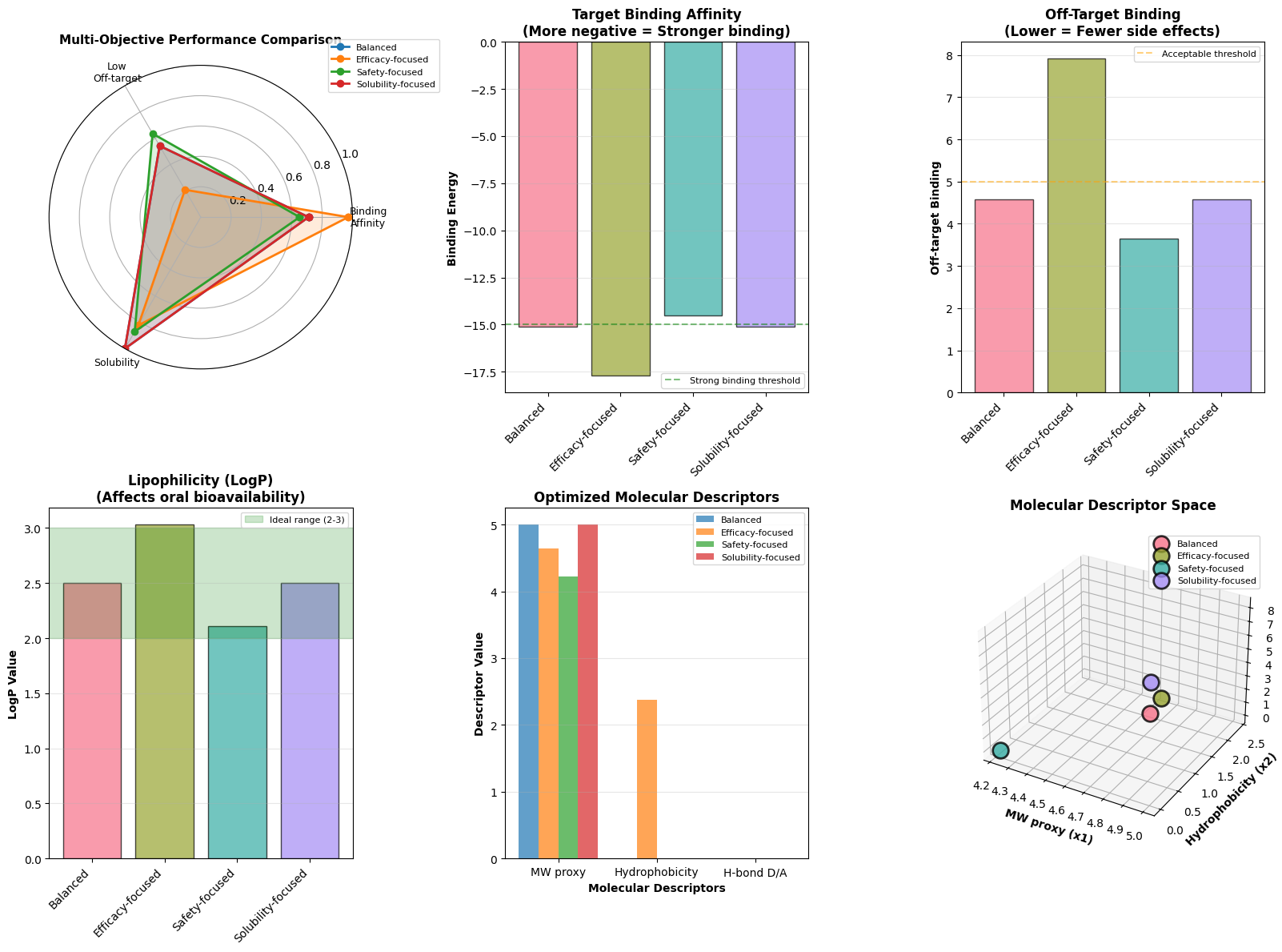
The code generates comprehensive visualizations:

1. Radar Chart: Shows the multi-dimensional performance of each scenario across all three objectives
2. Bar Charts: Compare individual metrics (affinity, off-target, LogP) across scenarios
3. Molecular Descriptors: Display the optimized values of $x_1$, $x_2$, $x_3$ for each approach
4. 3D Scatter Plot: Visualizes the solutions in the molecular descriptor space
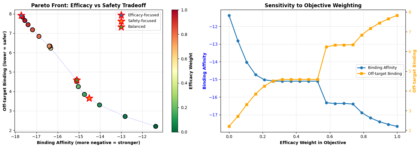
5. Pareto Front: Explores the fundamental tradeoff between efficacy and safety
6. Sensitivity Analysis: Shows how objective weights affect the optimal solution

5. Pareto Front Analysis

The second part generates 20 different solutions by varying the weight ratio between efficacy and safety (keeping solubility weight fixed). This creates a Pareto front showing the inherent tradeoff: you cannot simultaneously maximize binding affinity while minimizing off-target effects. The Pareto front helps decision-makers understand what compromises are necessary.

Expected Results and Interpretation

Execution Results

======================================================================
DRUG MOLECULAR DESIGN OPTIMIZATION RESULTS
======================================================================

Balanced Approach:
  Molecular descriptors: x1=5.000, x2=0.000, x3=0.000
  Binding affinity: -15.101 (more negative = stronger)
  Off-target binding: 4.579 (lower = fewer side effects)
  Solubility penalty: 0.000 (lower = better)
  LogP value: 2.500 (ideal: 2-3)

Efficacy-focused Approach:
  Molecular descriptors: x1=4.636, x2=2.378, x3=0.000
  Binding affinity: -17.715 (more negative = stronger)
  Off-target binding: 7.919 (lower = fewer side effects)
  Solubility penalty: 0.531 (lower = better)
  LogP value: 3.031 (ideal: 2-3)

Safety-focused Approach:
  Molecular descriptors: x1=4.224, x2=0.000, x3=0.000
  Binding affinity: -14.516 (more negative = stronger)
  Off-target binding: 3.647 (lower = fewer side effects)
  Solubility penalty: 0.388 (lower = better)
  LogP value: 2.112 (ideal: 2-3)

Solubility-focused Approach:
  Molecular descriptors: x1=5.000, x2=0.000, x3=0.000
  Binding affinity: -15.101 (more negative = stronger)
  Off-target binding: 4.579 (lower = fewer side effects)
  Solubility penalty: 0.000 (lower = better)
  LogP value: 2.500 (ideal: 2-3)

======================================================================

======================================================================
PARETO FRONT ANALYSIS: Efficacy vs Safety Tradeoff
======================================================================

Optimization complete! Graphs saved and displayed.
======================================================================

---

Graph Interpretation Guide

Radar Chart: The balanced approach should show a more uniform pentagon, while specialized approaches will be skewed toward their prioritized objective. This helps visualize multi-objective tradeoffs at a glance.

Binding Affinity Chart: Efficacy-focused scenarios should achieve the most negative (strongest) binding energies, typically around -15 to -17, while safety-focused approaches may sacrifice some binding strength.

Off-target Binding Chart: Safety-focused optimization should yield the lowest values (ideally below 5), reducing potential side effects. Efficacy-focused approaches may show higher off-target binding as a tradeoff.

LogP Chart: Solubility-focused scenarios should land closest to the green ideal range (2-3). Values outside this range indicate either poor water solubility (>3) or poor membrane permeability (<2).

Pareto Front: The curved relationship shows that improving efficacy inevitably increases off-target binding (and vice versa). The optimal drug design lies somewhere on this curve, depending on therapeutic priorities. For life-threatening diseases, we might accept more side effects for higher efficacy; for chronic conditions, we might prioritize safety.

Practical Implications

In real drug discovery:

1. Lead Optimization: This approach helps optimize lead compounds by systematically exploring the design space
2. Decision Support: Visualizations help medicinal chemists and project teams make informed decisions about which molecular modifications to pursue
3. Risk Assessment: Understanding tradeoffs early prevents late-stage failures due to poor ADME (Absorption, Distribution, Metabolism, Excretion) properties
4. Portfolio Management: Different scenarios could represent different drug candidates in a pipeline, each optimized for different therapeutic contexts

This methodology can be extended with:

• Real molecular descriptors from cheminformatics libraries (RDKit)
• Machine learning models trained on experimental data
• Additional objectives (metabolic stability, toxicity, synthetic accessibility)
• Constraint handling for drug-like properties (Lipinski’s Rule of Five)

The key insight is that drug design is fundamentally a multi-objective optimization problem where perfect solutions don’t exist—only optimal compromises based on therapeutic priorities.