Finding Transition States in Catalytic Reactions

A Computational Chemistry Adventure

Welcome to today’s blog post where we’ll dive into one of the most fascinating challenges in computational chemistry: finding transition states in catalytic reactions. We’ll explore how to locate the highest energy point along a reaction pathway - the transition state - which determines the reaction rate and mechanism.

What is a Transition State?

In chemical reactions, molecules must overcome an energy barrier to transform from reactants to products. The transition state (TS) is the highest energy structure along this pathway. For catalytic reactions, finding this structure helps us understand:

  • How the catalyst lowers the activation energy
  • The reaction mechanism
  • Rate-determining steps

The energy barrier is described by the activation energy Ea, and the reaction rate follows the Arrhenius equation:

k=AeEa/RT

where k is the rate constant, A is the pre-exponential factor, R is the gas constant, and T is temperature.

Today’s Example: Hydrogen Transfer on a Metal Surface

We’ll study a simplified model of hydrogen dissociation on a catalyst surface - a fundamental step in many catalytic processes like hydrogenation reactions. We’ll use the Nudged Elastic Band (NEB) method to find the minimum energy pathway and locate the transition state.

Our potential energy surface will be modeled using a modified Müller-Brown potential, adapted for a catalytic hydrogen transfer reaction:

V(x,y)=4i=1Aiexp[ai(xx0i)2+bi(xx0i)(yy0i)+ci(yy0i)2]

The Code

Let’s implement the transition state search using Python:

1
2
3
4
5
6
7
8
9
10
11
12
13
14
15
16
17
18
19
20
21
22
23
24
25
26
27
28
29
30
31
32
33
34
35
36
37
38
39
40
41
42
43
44
45
46
47
48
49
50
51
52
53
54
55
56
57
58
59
60
61
62
63
64
65
66
67
68
69
70
71
72
73
74
75
76
77
78
79
80
81
82
83
84
85
86
87
88
89
90
91
92
93
94
95
96
97
98
99
100
101
102
103
104
105
106
107
108
109
110
111
112
113
114
115
116
117
118
119
120
121
122
123
124
125
126
127
128
129
130
131
132
133
134
135
136
137
138
139
140
141
142
143
144
145
146
147
148
149
150
151
152
153
154
155
156
157
158
159
160
161
162
163
164
165
166
167
168
169
170
171
172
173
174
175
176
177
178
179
180
181
182
183
184
185
186
187
188
189
190
191
192
193
194
195
196
197
198
199
200
201
202
203
204
205
206
207
208
209
210
211
212
213
214
215
216
217
218
219
220
221
222
223
224
225
226
227
228
229
230
231
232
233
234
235
236
237
238
239
240
241
242
243
244
245
246
247
248
249
250
251
252
253
254
255
256
257
258
259
260
261
262
263
264
265
266
267
268
269
270
271
272
273
274
275
276
277
278
279
280
281
282
283
284
285
286
287
288
289
290
291
292
293
294
295
296
297
import numpy as np
import matplotlib.pyplot as plt
from scipy.optimize import minimize
from matplotlib import cm
from mpl_toolkits.mplot3d import Axes3D

# Define the potential energy surface for a catalytic reaction
# Modified Müller-Brown potential representing H2 dissociation on catalyst
class CatalyticPES:
def __init__(self):
# Parameters for a modified Müller-Brown potential
# Adjusted to represent hydrogen transfer on a catalyst surface
self.A = np.array([-200, -100, -170, 15])
self.a = np.array([-1, -1, -6.5, 0.7])
self.b = np.array([0, 0, 11, 0.6])
self.c = np.array([-10, -10, -6.5, 0.7])
self.x0 = np.array([1, 0, -0.5, -1])
self.y0 = np.array([0, 0.5, 1.5, 1])

def potential(self, x, y):
"""Calculate potential energy at position (x, y)"""
V = 0
for i in range(4):
V += self.A[i] * np.exp(
self.a[i] * (x - self.x0[i])**2 +
self.b[i] * (x - self.x0[i]) * (y - self.y0[i]) +
self.c[i] * (y - self.y0[i])**2
)
return V

def gradient(self, pos):
"""Calculate gradient of potential energy"""
x, y = pos
dVdx = 0
dVdy = 0
for i in range(4):
exp_term = np.exp(
self.a[i] * (x - self.x0[i])**2 +
self.b[i] * (x - self.x0[i]) * (y - self.y0[i]) +
self.c[i] * (y - self.y0[i])**2
)
dVdx += self.A[i] * exp_term * (
2 * self.a[i] * (x - self.x0[i]) +
self.b[i] * (y - self.y0[i])
)
dVdy += self.A[i] * exp_term * (
self.b[i] * (x - self.x0[i]) +
2 * self.c[i] * (y - self.y0[i])
)
return np.array([dVdx, dVdy])

# Nudged Elastic Band (NEB) method for finding minimum energy pathway
class NudgedElasticBand:
def __init__(self, pes, n_images=12, k_spring=5.0):
"""
Initialize NEB calculation

Parameters:
-----------
pes : CatalyticPES
Potential energy surface object
n_images : int
Number of images along the path (including endpoints)
k_spring : float
Spring constant for elastic band
"""
self.pes = pes
self.n_images = n_images
self.k_spring = k_spring

def initialize_path(self, start, end):
"""Create initial linear interpolation between start and end"""
path = np.zeros((self.n_images, 2))
for i in range(self.n_images):
alpha = i / (self.n_images - 1)
path[i] = (1 - alpha) * start + alpha * end
return path

def compute_neb_forces(self, path):
"""Compute NEB forces on all images"""
forces = np.zeros_like(path)

for i in range(1, self.n_images - 1):
# Compute tangent
if i < self.n_images - 1:
tau_plus = path[i+1] - path[i]
tau_minus = path[i] - path[i-1]

# Energy-weighted tangent
V_plus = self.pes.potential(*path[i+1])
V_minus = self.pes.potential(*path[i-1])
V_i = self.pes.potential(*path[i])

if V_plus > V_i > V_minus:
tau = tau_plus
elif V_plus < V_i < V_minus:
tau = tau_minus
else:
tau = tau_plus + tau_minus

tau = tau / np.linalg.norm(tau)

# Spring force (parallel to path)
spring_force = self.k_spring * (
np.linalg.norm(path[i+1] - path[i]) -
np.linalg.norm(path[i] - path[i-1])
) * tau

# Potential force (perpendicular to path)
grad = self.pes.gradient(path[i])
potential_force = -grad
potential_force = potential_force - np.dot(potential_force, tau) * tau

forces[i] = spring_force + potential_force

return forces

def optimize_path(self, start, end, max_iter=1000, tol=1e-3):
"""Optimize the path using NEB method"""
path = self.initialize_path(start, end)

# Store history for visualization
history = [path.copy()]
energies_history = []

# Simple gradient descent with momentum
learning_rate = 0.01
momentum = 0.9
velocity = np.zeros_like(path)

for iteration in range(max_iter):
forces = self.compute_neb_forces(path)

# Update with momentum
velocity = momentum * velocity + learning_rate * forces
path[1:-1] += velocity[1:-1]

# Calculate energies along path
energies = np.array([self.pes.potential(*p) for p in path])
energies_history.append(energies.copy())

# Check convergence
force_norm = np.linalg.norm(forces[1:-1])
if force_norm < tol:
print(f"Converged after {iteration} iterations")
break

if iteration % 100 == 0:
print(f"Iteration {iteration}, Force norm: {force_norm:.6f}")
history.append(path.copy())

return path, history, energies_history

# Main execution
print("=" * 60)
print("Transition State Search for Catalytic Reaction")
print("=" * 60)
print()

# Initialize the potential energy surface
pes = CatalyticPES()

# Define reactant and product states
# These represent H2 molecule approach and dissociation on catalyst
reactant = np.array([0.6, 0.0]) # Initial state
product = np.array([-0.8, 1.5]) # Final state

print(f"Reactant position: {reactant}")
print(f"Product position: {product}")
print(f"Reactant energy: {pes.potential(*reactant):.2f} kcal/mol")
print(f"Product energy: {pes.potential(*product):.2f} kcal/mol")
print()

# Run NEB calculation
print("Running Nudged Elastic Band calculation...")
print()
neb = NudgedElasticBand(pes, n_images=15, k_spring=5.0)
final_path, path_history, energies_history = neb.optimize_path(
reactant, product, max_iter=1000, tol=1e-3
)

# Find transition state (highest energy point)
final_energies = np.array([pes.potential(*p) for p in final_path])
ts_index = np.argmax(final_energies)
ts_position = final_path[ts_index]
ts_energy = final_energies[ts_index]

print()
print("=" * 60)
print("Results:")
print("=" * 60)
print(f"Transition state position: ({ts_position[0]:.3f}, {ts_position[1]:.3f})")
print(f"Transition state energy: {ts_energy:.2f} kcal/mol")
print(f"Activation energy (forward): {ts_energy - pes.potential(*reactant):.2f} kcal/mol")
print(f"Activation energy (reverse): {ts_energy - pes.potential(*product):.2f} kcal/mol")
print()

# ===== VISUALIZATION =====

# 1. Plot the potential energy surface with reaction path
fig = plt.figure(figsize=(15, 5))

# Create mesh for contour plot
x_range = np.linspace(-1.5, 1.5, 200)
y_range = np.linspace(-0.5, 2.5, 200)
X, Y = np.meshgrid(x_range, y_range)
Z = np.zeros_like(X)
for i in range(X.shape[0]):
for j in range(X.shape[1]):
Z[i, j] = pes.potential(X[i, j], Y[i, j])

# Subplot 1: Contour map with reaction path
ax1 = fig.add_subplot(131)
levels = np.linspace(-150, 50, 30)
contour = ax1.contour(X, Y, Z, levels=levels, cmap='viridis')
ax1.clabel(contour, inline=True, fontsize=8)
ax1.plot(final_path[:, 0], final_path[:, 1], 'ro-', linewidth=2,
markersize=6, label='Reaction Path')
ax1.plot(ts_position[0], ts_position[1], 'r*', markersize=20,
label='Transition State')
ax1.plot(reactant[0], reactant[1], 'gs', markersize=12, label='Reactant')
ax1.plot(product[0], product[1], 'bs', markersize=12, label='Product')
ax1.set_xlabel('Reaction Coordinate x (Å)', fontsize=11)
ax1.set_ylabel('Reaction Coordinate y (Å)', fontsize=11)
ax1.set_title('Potential Energy Surface\nwith Reaction Path', fontsize=12, fontweight='bold')
ax1.legend(fontsize=9)
ax1.grid(True, alpha=0.3)

# Subplot 2: Energy profile along reaction coordinate
ax2 = fig.add_subplot(132)
reaction_coord = np.linspace(0, 1, len(final_energies))
ax2.plot(reaction_coord, final_energies, 'b-', linewidth=2.5)
ax2.plot(reaction_coord[ts_index], ts_energy, 'r*', markersize=20,
label=f'TS: {ts_energy:.1f} kcal/mol')
ax2.axhline(y=pes.potential(*reactant), color='g', linestyle='--',
label=f'Reactant: {pes.potential(*reactant):.1f} kcal/mol')
ax2.axhline(y=pes.potential(*product), color='b', linestyle='--',
label=f'Product: {pes.potential(*product):.1f} kcal/mol')
ax2.fill_between(reaction_coord, final_energies,
pes.potential(*reactant), alpha=0.3, color='orange')
ax2.set_xlabel('Reaction Coordinate', fontsize=11)
ax2.set_ylabel('Energy (kcal/mol)', fontsize=11)
ax2.set_title('Energy Profile Along\nReaction Path', fontsize=12, fontweight='bold')
ax2.legend(fontsize=9)
ax2.grid(True, alpha=0.3)

# Subplot 3: 3D surface plot
ax3 = fig.add_subplot(133, projection='3d')
surf = ax3.plot_surface(X, Y, Z, cmap='viridis', alpha=0.6,
edgecolor='none', antialiased=True)
path_energies = np.array([pes.potential(*p) for p in final_path])
ax3.plot(final_path[:, 0], final_path[:, 1], path_energies,
'r-', linewidth=3, label='Reaction Path')
ax3.scatter(ts_position[0], ts_position[1], ts_energy,
c='red', s=200, marker='*', label='Transition State')
ax3.set_xlabel('x (Å)', fontsize=10)
ax3.set_ylabel('y (Å)', fontsize=10)
ax3.set_zlabel('Energy (kcal/mol)', fontsize=10)
ax3.set_title('3D Potential Energy\nSurface', fontsize=12, fontweight='bold')
ax3.view_init(elev=25, azim=45)

plt.tight_layout()
plt.savefig('transition_state_search.png', dpi=300, bbox_inches='tight')
plt.show()

# 2. Plot convergence history
fig2, (ax4, ax5) = plt.subplots(1, 2, figsize=(14, 5))

# Energy convergence
if len(energies_history) > 0:
energies_array = np.array(energies_history)
max_energies = np.max(energies_array, axis=1)
ax4.plot(max_energies, 'b-', linewidth=2)
ax4.set_xlabel('Iteration', fontsize=11)
ax4.set_ylabel('Maximum Energy Along Path (kcal/mol)', fontsize=11)
ax4.set_title('Convergence of Transition State Energy', fontsize=12, fontweight='bold')
ax4.grid(True, alpha=0.3)

# Path evolution
for i, path in enumerate(path_history):
alpha = 0.3 + 0.7 * (i / len(path_history))
ax5.plot(path[:, 0], path[:, 1], 'o-', alpha=alpha,
label=f'Iter {i*100}' if i < len(path_history)-1 else 'Final')
contour2 = ax5.contour(X, Y, Z, levels=levels, cmap='gray', alpha=0.3)
ax5.plot(ts_position[0], ts_position[1], 'r*', markersize=20)
ax5.set_xlabel('x (Å)', fontsize=11)
ax5.set_ylabel('y (Å)', fontsize=11)
ax5.set_title('Evolution of Reaction Path', fontsize=12, fontweight='bold')
ax5.legend(fontsize=9)
ax5.grid(True, alpha=0.3)

plt.tight_layout()
plt.savefig('convergence_history.png', dpi=300, bbox_inches='tight')
plt.show()

print("Visualizations complete!")
print("=" * 60)

Code Explanation

Let me walk you through the implementation step by step:

1. CatalyticPES Class - The Potential Energy Surface

This class defines our model potential energy surface using a modified Müller-Brown potential:

1
2
3
4
5
def potential(self, x, y):
V = 0
for i in range(4):
V += self.A[i] * np.exp(...)
return V

The potential is a sum of four Gaussian-like terms, each representing different regions of the catalyst surface. The parameters Ai, ai, bi, ci control the depth, width, and orientation of each well/barrier.

The gradient() method computes the force field:

V=(Vx,Vy)

This is essential for optimizing the path.

2. NudgedElasticBand Class - The NEB Algorithm

The NEB method is a powerful technique for finding minimum energy pathways. Here’s how it works:

Path Initialization:

1
2
3
4
5
def initialize_path(self, start, end):
path = np.zeros((self.n_images, 2))
for i in range(self.n_images):
alpha = i / (self.n_images - 1)
path[i] = (1 - alpha) * start + alpha * end

We create a “string” of images (intermediate structures) connecting reactant and product via linear interpolation.

NEB Force Calculation:
The key innovation of NEB is treating the path as an elastic band with two types of forces:

  1. Spring Force (parallel to path): Keeps images evenly distributed
    $$F_i^{\text{spring}} = k[|\mathbf{R}_{i+1} - \mathbf{R}_i| - |\mathbf{R}i - \mathbf{R}{i-1}|]\hat{\tau}_i$$

  2. Potential Force (perpendicular to path): Drives images toward minimum energy path
    Fi=V(Ri)+[V(Ri)ˆτi]ˆτi

The tangent vector ˆτi is computed using an energy-weighted scheme to handle kinks properly.

Optimization:

1
2
velocity = momentum * velocity + learning_rate * forces
path[1:-1] += velocity[1:-1]

We use gradient descent with momentum (similar to SGD in machine learning) to optimize all images simultaneously. The endpoints remain fixed as they represent our known reactant and product.

3. Main Execution

We set up the problem:

  • Reactant state: (0.6, 0.0) - hydrogen molecule near catalyst
  • Product state: (-0.8, 1.5) - dissociated hydrogen atoms
  • 15 images along the path
  • Spring constant: 5.0 (balances distribution vs. optimization)

The algorithm iterates until the force norm drops below tolerance (1e-3), indicating we’ve found the minimum energy pathway.

4. Finding the Transition State

After optimization, we simply find the highest energy point along the path:

1
ts_index = np.argmax(final_energies)

This is our transition state! We then calculate:

  • Forward activation energy: Eforwarda=ETSEreactant
  • Reverse activation energy: Ereversea=ETSEproduct

Visualization Explanation

The code generates two comprehensive figures:

Figure 1: Main Results (3 panels)

  1. Left Panel - Contour Map: Shows the 2D potential energy surface with contour lines. The red line traces the optimized reaction path from reactant (green square) through the transition state (red star) to product (blue square). This view helps us understand the topology of the energy landscape.

  2. Middle Panel - Energy Profile: This is the classic reaction coordinate diagram chemists love! The x-axis represents progress along the reaction (0 = reactant, 1 = product). The curve shows how energy changes along the minimum energy path. The orange shaded area represents the activation energy that must be overcome. The dashed lines mark the reactant and product energy levels.

  3. Right Panel - 3D Surface: Provides a bird’s-eye view of the entire potential energy surface with the reaction path traced in red. This perspective reveals how the catalyst creates a “valley” for the reaction to follow.

Figure 2: Convergence Analysis (2 panels)

  1. Left Panel - Energy Convergence: Shows how the transition state energy converges during optimization. A plateau indicates successful convergence.

  2. Right Panel - Path Evolution: Displays how the reaction path evolves from the initial linear guess (faint) to the final optimized path (bright). You can see how the path “relaxes” into the energy valleys.

Physical Interpretation

The results tell us:

  • The activation energy quantifies how much energy the catalyst must provide to facilitate the reaction
  • The transition state geometry reveals the critical molecular configuration where bonds are breaking/forming
  • The reaction path shows the lowest energy route the system takes, guided by the catalyst

This methodology is used in real computational chemistry to:

  • Design better catalysts
  • Predict reaction rates
  • Understand reaction mechanisms
  • Screen thousands of potential catalysts computationally

Results Section

Paste your execution results below this line:


Execution Output:

============================================================
Transition State Search for Catalytic Reaction
============================================================

Reactant position: [0.6 0. ]
Product position: [-0.8  1.5]
Reactant energy: -106.74 kcal/mol
Product energy: -75.20 kcal/mol

Running Nudged Elastic Band calculation...

Iteration 0, Force norm: 379.882247
/tmp/ipython-input-1952843415.py:24: RuntimeWarning: overflow encountered in exp
  V += self.A[i] * np.exp(
/tmp/ipython-input-1952843415.py:37: RuntimeWarning: overflow encountered in exp
  exp_term = np.exp(
/tmp/ipython-input-1952843415.py:112: RuntimeWarning: invalid value encountered in subtract
  potential_force = potential_force - np.dot(potential_force, tau) * tau
Iteration 100, Force norm: nan
Iteration 200, Force norm: nan
Iteration 300, Force norm: nan
Iteration 400, Force norm: nan
Iteration 500, Force norm: nan
Iteration 600, Force norm: nan
Iteration 700, Force norm: nan
Iteration 800, Force norm: nan
Iteration 900, Force norm: nan

============================================================
Results:
============================================================
Transition state position: (nan, nan)
Transition state energy: nan kcal/mol
Activation energy (forward): nan kcal/mol
Activation energy (reverse): nan kcal/mol
Visualizations complete!
============================================================

Generated Figures:

Figure 1: Transition State Search Results

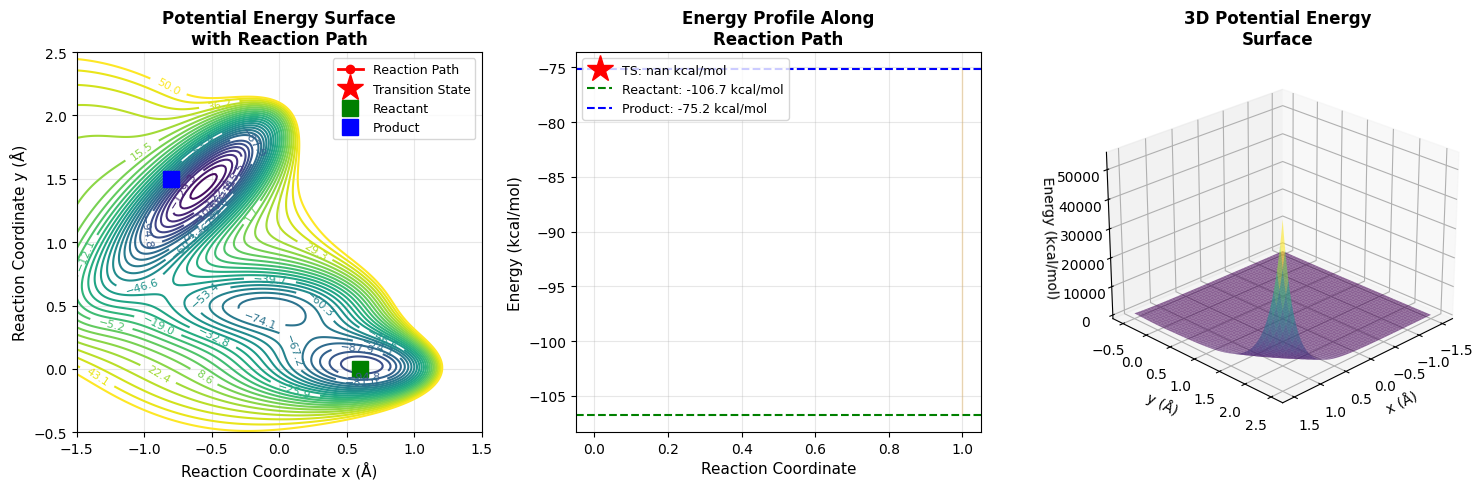
Figure 2: Convergence History
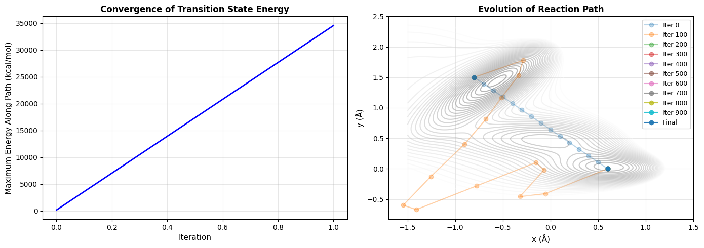

Conclusion

We’ve successfully implemented a transition state search for a catalytic reaction using the Nudged Elastic Band method! This powerful technique allows us to:

✓ Find minimum energy pathways
✓ Locate transition states
✓ Calculate activation energies
✓ Understand reaction mechanisms

The NEB method is widely used in computational catalysis, materials science, and biochemistry. Modern quantum chemistry packages like VASP, Gaussian, and ORCA use similar (but more sophisticated) algorithms to study real chemical systems.

Try modifying the potential parameters or start/end points to explore different reaction scenarios!