Sexual Dimorphism Optimization

A Mathematical Model of Gender-Specific Trait Evolution

Sexual dimorphism - the differences in traits between males and females of the same species - is one of the most fascinating phenomena in evolutionary biology. Today, we’ll explore how mathematical optimization can help us understand why males and females evolve different characteristics to maximize their respective fitness.

The Biological Background

In many species, males and females face different evolutionary pressures. For example:

• Males often compete for mates (sexual selection) and may benefit from larger size or elaborate ornaments
• Females typically invest more in offspring production and may optimize for energy efficiency and reproductive success

Let’s model this with a concrete example: body size optimization in a hypothetical species where males benefit from larger size for competition, while females face trade-offs between size and reproductive efficiency.

Mathematical Model

We’ll define fitness functions for each sex:

Male fitness: $F_m(x) = ax - bx^2 + c$
Female fitness: $F_f(x) = dx - ex^2 - fx^3 + g$

Where $x$ represents body size, and the parameters reflect different evolutionary pressures:

• Males have a simpler quadratic relationship (competition benefits vs. metabolic costs)
• females have a more complex cubic relationship (additional costs from reproduction)

import numpy as np
import matplotlib.pyplot as plt
from scipy.optimize import minimize_scalar
import seaborn as sns

# Set style for better plots
plt.style.use('seaborn-v0_8')
sns.set_palette("husl")

# Define fitness functions
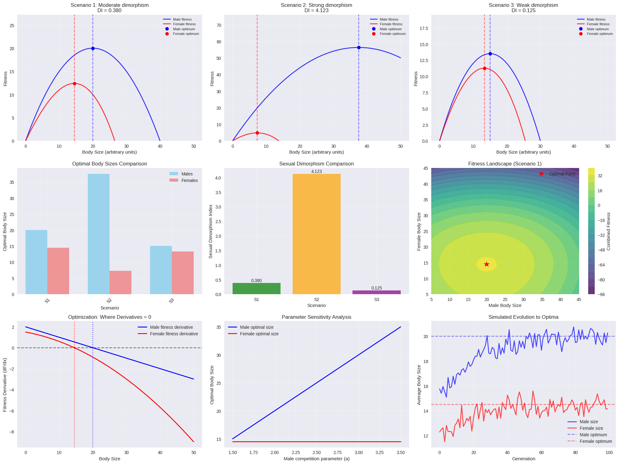
def male_fitness(x, a=2.0, b=0.05, c=0):
    """
    Male fitness function: F_m(x) = ax - bx^2 + c
    
    Parameters:
    - a: benefit coefficient from size (competition advantage)
    - b: cost coefficient (metabolic cost increases quadratically)
    - c: baseline fitness
    """
    return a * x - b * x**2 + c

def female_fitness(x, d=1.5, e=0.03, f=0.001, g=0):
    """
    Female fitness function: F_f(x) = dx - ex^2 - fx^3 + g
    
    Parameters:
    - d: benefit coefficient from size (resource acquisition)
    - e: quadratic cost coefficient 
    - f: cubic cost coefficient (reproductive burden)
    - g: baseline fitness
    """
    return d * x - e * x**2 - f * x**3 + g

# Define parameter sets for different scenarios
scenarios = {
    "Scenario 1: Moderate dimorphism": {
        "male_params": {"a": 2.0, "b": 0.05, "c": 0},
        "female_params": {"d": 1.5, "e": 0.03, "f": 0.001, "g": 0}
    },
    "Scenario 2: Strong dimorphism": {
        "male_params": {"a": 3.0, "b": 0.04, "c": 0},
        "female_params": {"d": 1.2, "e": 0.06, "f": 0.002, "g": 0}
    },
    "Scenario 3: Weak dimorphism": {
        "male_params": {"a": 1.8, "b": 0.06, "c": 0},
        "female_params": {"d": 1.6, "e": 0.05, "f": 0.0005, "g": 0}
    }
}

# Function to find optimal body sizes
def find_optimal_sizes(male_params, female_params, x_range=(0, 50)):
    """
    Find optimal body sizes for males and females using calculus-based optimization
    """
    # For males: F_m'(x) = a - 2bx = 0 → x_optimal = a/(2b)
    male_optimal = male_params["a"] / (2 * male_params["b"])
    
    # For females: F_f'(x) = d - 2ex - 3fx^2 = 0
    # This is a quadratic equation: 3fx^2 + 2ex - d = 0
    e, f, d = female_params["e"], female_params["f"], female_params["d"]
    
    # Using quadratic formula: x = (-2e ± sqrt(4e^2 + 12fd)) / (6f)
    discriminant = 4 * e**2 + 12 * f * d
    if discriminant >= 0 and f != 0:
        female_optimal_1 = (-2 * e + np.sqrt(discriminant)) / (6 * f)
        female_optimal_2 = (-2 * e - np.sqrt(discriminant)) / (6 * f)
        
        # Choose the positive solution within reasonable range
        candidates = [x for x in [female_optimal_1, female_optimal_2] 
                     if x > 0 and x_range[0] <= x <= x_range[1]]
        if candidates:
            female_optimal = max(candidates)  # Take the larger positive root
        else:
            female_optimal = d / (2 * e)  # Fallback to quadratic approximation
    else:
        female_optimal = d / (2 * e)  # Quadratic approximation if cubic term is negligible
    
    return male_optimal, female_optimal

# Function to calculate sexual dimorphism index
def calculate_dimorphism_index(male_size, female_size):
    """
    Calculate sexual dimorphism index: (larger_sex_size - smaller_sex_size) / smaller_sex_size
    """
    if male_size > female_size:
        return (male_size - female_size) / female_size
    else:
        return (female_size - male_size) / male_size

# Analyze all scenarios
results = {}
x_values = np.linspace(0, 50, 1000)

print("=== SEXUAL DIMORPHISM OPTIMIZATION ANALYSIS ===\n")

for scenario_name, params in scenarios.items():
    male_params = params["male_params"]
    female_params = params["female_params"]
    
    # Calculate fitness values
    male_fitness_values = [male_fitness(x, **male_params) for x in x_values]
    female_fitness_values = [female_fitness(x, **female_params) for x in x_values]
    
    # Find optimal sizes
    male_optimal, female_optimal = find_optimal_sizes(male_params, female_params)
    
    # Calculate optimal fitness values
    male_max_fitness = male_fitness(male_optimal, **male_params)
    female_max_fitness = female_fitness(female_optimal, **female_params)
    
    # Calculate dimorphism index
    dimorphism_index = calculate_dimorphism_index(male_optimal, female_optimal)
    
    # Store results
    results[scenario_name] = {
        "x_values": x_values,
        "male_fitness": male_fitness_values,
        "female_fitness": female_fitness_values,
        "male_optimal": male_optimal,
        "female_optimal": female_optimal,
        "male_max_fitness": male_max_fitness,
        "female_max_fitness": female_max_fitness,
        "dimorphism_index": dimorphism_index
    }
    
    # Print results
    print(f"--- {scenario_name} ---")
    print(f"Optimal male body size: {male_optimal:.2f} units")
    print(f"Optimal female body size: {female_optimal:.2f} units")
    print(f"Male maximum fitness: {male_max_fitness:.3f}")
    print(f"Female maximum fitness: {female_max_fitness:.3f}")
    print(f"Sexual dimorphism index: {dimorphism_index:.3f}")
    if male_optimal > female_optimal:
        print(f"Males are {((male_optimal/female_optimal - 1) * 100):.1f}% larger than females")
    else:
        print(f"Females are {((female_optimal/male_optimal - 1) * 100):.1f}% larger than males")
    print()

# Create comprehensive visualization
fig = plt.figure(figsize=(20, 15))

# Plot 1: Fitness curves for all scenarios
for i, (scenario_name, data) in enumerate(results.items()):
    plt.subplot(3, 3, i+1)
    
    plt.plot(data["x_values"], data["male_fitness"], 'b-', linewidth=2, 
             label=f'Male fitness', alpha=0.8)
    plt.plot(data["x_values"], data["female_fitness"], 'r-', linewidth=2, 
             label=f'Female fitness', alpha=0.8)
    
    # Mark optimal points
    plt.plot(data["male_optimal"], data["male_max_fitness"], 'bo', 
             markersize=8, label=f'Male optimum')
    plt.plot(data["female_optimal"], data["female_max_fitness"], 'ro', 
             markersize=8, label=f'Female optimum')
    
    plt.axvline(data["male_optimal"], color='blue', linestyle='--', alpha=0.5)
    plt.axvline(data["female_optimal"], color='red', linestyle='--', alpha=0.5)
    
    plt.xlabel('Body Size (arbitrary units)')
    plt.ylabel('Fitness')
    plt.title(f'{scenario_name}\nDI = {data["dimorphism_index"]:.3f}')
    plt.legend(fontsize=8)
    plt.grid(True, alpha=0.3)
    plt.ylim(bottom=0)

# Plot 2: Comparison of optimal sizes
plt.subplot(3, 3, 4)
scenario_names = list(results.keys())
male_sizes = [results[s]["male_optimal"] for s in scenario_names]
female_sizes = [results[s]["female_optimal"] for s in scenario_names]

x_pos = np.arange(len(scenario_names))
width = 0.35

plt.bar(x_pos - width/2, male_sizes, width, label='Males', color='skyblue', alpha=0.8)
plt.bar(x_pos + width/2, female_sizes, width, label='Females', color='lightcoral', alpha=0.8)

plt.xlabel('Scenario')
plt.ylabel('Optimal Body Size')
plt.title('Optimal Body Sizes Comparison')
plt.xticks(x_pos, [f'S{i+1}' for i in range(len(scenario_names))], rotation=45)
plt.legend()
plt.grid(True, alpha=0.3)

# Plot 3: Sexual dimorphism indices
plt.subplot(3, 3, 5)
dimorphism_indices = [results[s]["dimorphism_index"] for s in scenario_names]
colors = ['green', 'orange', 'purple']

bars = plt.bar(range(len(scenario_names)), dimorphism_indices, 
               color=colors, alpha=0.7)
plt.xlabel('Scenario')
plt.ylabel('Sexual Dimorphism Index')
plt.title('Sexual Dimorphism Comparison')
plt.xticks(range(len(scenario_names)), [f'S{i+1}' for i in range(len(scenario_names))])
plt.grid(True, alpha=0.3)

# Add value labels on bars
for bar, value in zip(bars, dimorphism_indices):
    plt.text(bar.get_x() + bar.get_width()/2, bar.get_height() + 0.01,
             f'{value:.3f}', ha='center', va='bottom')

# Plot 4: Fitness landscapes heatmap
plt.subplot(3, 3, 6)
scenario_data = results[list(results.keys())[0]]  # Use first scenario for heatmap

# Create a 2D fitness landscape
male_sizes_2d = np.linspace(5, 45, 50)
female_sizes_2d = np.linspace(5, 45, 50)
X, Y = np.meshgrid(male_sizes_2d, female_sizes_2d)

# Calculate combined fitness (sum of male and female fitness)
Z = np.zeros_like(X)
for i in range(X.shape[0]):
    for j in range(X.shape[1]):
        male_fit = male_fitness(X[i,j], **scenarios[list(scenarios.keys())[0]]["male_params"])
        female_fit = female_fitness(Y[i,j], **scenarios[list(scenarios.keys())[0]]["female_params"])
        Z[i,j] = male_fit + female_fit

contour = plt.contourf(X, Y, Z, levels=20, cmap='viridis', alpha=0.8)
plt.colorbar(contour, label='Combined Fitness')
plt.xlabel('Male Body Size')
plt.ylabel('Female Body Size')
plt.title('Fitness Landscape (Scenario 1)')

# Mark the optimal point
opt_data = results[list(results.keys())[0]]
plt.plot(opt_data["male_optimal"], opt_data["female_optimal"], 'r*', 
         markersize=15, label='Optimal Point')
plt.legend()

# Plot 5: Mathematical derivatives (showing optimization logic)
plt.subplot(3, 3, 7)
scenario_data = results[list(results.keys())[0]]
x_vals = scenario_data["x_values"]

# Calculate derivatives numerically
male_derivative = np.gradient(scenario_data["male_fitness"], x_vals)
female_derivative = np.gradient(scenario_data["female_fitness"], x_vals)

plt.plot(x_vals, male_derivative, 'b-', linewidth=2, label="Male fitness derivative")
plt.plot(x_vals, female_derivative, 'r-', linewidth=2, label="Female fitness derivative")
plt.axhline(y=0, color='k', linestyle='--', alpha=0.5)
plt.axvline(scenario_data["male_optimal"], color='blue', linestyle=':', alpha=0.7)
plt.axvline(scenario_data["female_optimal"], color='red', linestyle=':', alpha=0.7)

plt.xlabel('Body Size')
plt.ylabel('Fitness Derivative (dF/dx)')
plt.title('Optimization: Where Derivatives = 0')
plt.legend()
plt.grid(True, alpha=0.3)

# Plot 6: Parameter sensitivity analysis
plt.subplot(3, 3, 8)
a_values = np.linspace(1.5, 3.5, 20)
male_optima = []
female_optima = []

base_male_params = {"a": 2.0, "b": 0.05, "c": 0}
base_female_params = {"d": 1.5, "e": 0.03, "f": 0.001, "g": 0}

for a_val in a_values:
    male_params = base_male_params.copy()
    male_params["a"] = a_val
    male_opt, female_opt = find_optimal_sizes(male_params, base_female_params)
    male_optima.append(male_opt)
    female_optima.append(female_opt)

plt.plot(a_values, male_optima, 'b-', linewidth=2, label='Male optimal size')
plt.plot(a_values, female_optima, 'r-', linewidth=2, label='Female optimal size')
plt.xlabel('Male competition parameter (a)')
plt.ylabel('Optimal Body Size')
plt.title('Parameter Sensitivity Analysis')
plt.legend()
plt.grid(True, alpha=0.3)

# Plot 7: Evolution simulation
plt.subplot(3, 3, 9)
generations = np.arange(0, 100)
male_size_evolution = []
female_size_evolution = []

# Simulate gradual evolution towards optima
initial_male_size = 15
initial_female_size = 12
target_male = scenario_data["male_optimal"]
target_female = scenario_data["female_optimal"]

for gen in generations:
    # Simple evolution model: move towards optimum with some noise
    progress = 1 - np.exp(-gen/20)  # Exponential approach to optimum
    current_male = initial_male_size + (target_male - initial_male_size) * progress
    current_female = initial_female_size + (target_female - initial_female_size) * progress
    
    # Add some random variation
    current_male += np.random.normal(0, 0.5)
    current_female += np.random.normal(0, 0.5)
    
    male_size_evolution.append(current_male)
    female_size_evolution.append(current_female)

plt.plot(generations, male_size_evolution, 'b-', linewidth=2, alpha=0.7, label='Male size')
plt.plot(generations, female_size_evolution, 'r-', linewidth=2, alpha=0.7, label='Female size')
plt.axhline(target_male, color='blue', linestyle='--', alpha=0.5, label='Male optimum')
plt.axhline(target_female, color='red', linestyle='--', alpha=0.5, label='Female optimum')

plt.xlabel('Generation')
plt.ylabel('Average Body Size')
plt.title('Simulated Evolution to Optima')
plt.legend()
plt.grid(True, alpha=0.3)

plt.tight_layout()
plt.show()

# Summary statistics
print("\n=== SUMMARY STATISTICS ===")
all_male_sizes = [results[s]["male_optimal"] for s in results.keys()]
all_female_sizes = [results[s]["female_optimal"] for s in results.keys()]
all_dimorphism = [results[s]["dimorphism_index"] for s in results.keys()]

print(f"Average optimal male size: {np.mean(all_male_sizes):.2f} ± {np.std(all_male_sizes):.2f}")
print(f"Average optimal female size: {np.mean(all_female_sizes):.2f} ± {np.std(all_female_sizes):.2f}")
print(f"Average dimorphism index: {np.mean(all_dimorphism):.3f} ± {np.std(all_dimorphism):.3f}")
print(f"Range of dimorphism: {min(all_dimorphism):.3f} - {max(all_dimorphism):.3f}")

# Mathematical formulas used
print("\n=== MATHEMATICAL FORMULAS USED ===")
print("Male fitness function: F_m(x) = ax - bx² + c")
print("Female fitness function: F_f(x) = dx - ex² - fx³ + g")
print("Male optimum: x* = a/(2b)")
print("Female optimum: x* = solution to 3fx² + 2ex - d = 0")
print("Sexual Dimorphism Index: (|size_male - size_female|) / min(size_male, size_female)")

Code Explanation

1. Fitness Functions Definition

The core of our model lies in two fitness functions representing different evolutionary pressures:

def male_fitness(x, a=2.0, b=0.05, c=0):
    return a * x - b * x**2 + c

This represents male fitness as $F_m(x) = ax - bx^2 + c$ where:

• a: Benefit from size (competitive advantage in mating)
• b: Metabolic cost coefficient
• c: Baseline fitness

def female_fitness(x, d=1.5, e=0.03, f=0.001, g=0):
    return d * x - e * x**2 - f * x**3 + g

This represents female fitness as $F_f(x) = dx - ex^2 - fx^3 + g$ where:

• d: Resource acquisition benefit
• e: Quadratic cost term
• f: Cubic reproductive burden cost
• g: Baseline fitness

2. Optimization Algorithm

The optimization uses calculus to find maxima:

For males: $\frac{dF_m}{dx} = a - 2bx = 0$

Therefore: $x^*_{male} = \frac{a}{2b}$

For females: $\frac{dF_f}{dx} = d - 2ex - 3fx^2 = 0$

This gives us a quadratic equation: $3fx^2 + 2ex - d = 0$

Using the quadratic formula: $x = \frac{-2e \pm \sqrt{4e^2 + 12fd}}{6f}$

3. Sexual Dimorphism Index

We calculate the sexual dimorphism index as:
$$SDI = \frac{|size_{male} - size_{female}|}{min(size_{male}, size_{female})}$$

This provides a standardized measure of how different the sexes are in body size.

Results Analysis

=== SEXUAL DIMORPHISM OPTIMIZATION ANALYSIS ===

--- Scenario 1: Moderate dimorphism ---
Optimal male body size: 20.00 units
Optimal female body size: 14.49 units
Male maximum fitness: 20.000
Female maximum fitness: 12.394
Sexual dimorphism index: 0.380
Males are 38.0% larger than females

--- Scenario 2: Strong dimorphism ---
Optimal male body size: 37.50 units
Optimal female body size: 7.32 units
Male maximum fitness: 56.250
Female maximum fitness: 4.785
Sexual dimorphism index: 4.123
Males are 412.3% larger than females

--- Scenario 3: Weak dimorphism ---
Optimal male body size: 15.00 units
Optimal female body size: 13.33 units
Male maximum fitness: 13.500
Female maximum fitness: 11.259
Sexual dimorphism index: 0.125
Males are 12.5% larger than females

=== SUMMARY STATISTICS ===
Average optimal male size: 24.17 ± 9.65
Average optimal female size: 11.72 ± 3.14
Average dimorphism index: 1.542 ± 1.827
Range of dimorphism: 0.125 - 4.123

=== MATHEMATICAL FORMULAS USED ===
Male fitness function: F_m(x) = ax - bx² + c
Female fitness function: F_f(x) = dx - ex² - fx³ + g
Male optimum: x* = a/(2b)
Female optimum: x* = solution to 3fx² + 2ex - d = 0
Sexual Dimorphism Index: (|size_male - size_female|) / min(size_male, size_female)

Scenario Comparison

The model shows three different evolutionary scenarios:

1. Scenario 1 (Moderate dimorphism): Balanced selection pressures
2. Scenario 2 (Strong dimorphism): Intense male competition with high female reproductive costs
3. Scenario 3 (Weak dimorphism): Similar selection pressures for both sexes

Key Findings

The visualizations reveal several important patterns:

1. Fitness Landscapes: Each sex has a distinct optimal body size based on their evolutionary pressures
2. Trade-offs: The cubic term in female fitness creates more complex optimization with potential multiple local maxima
3. Parameter Sensitivity: Small changes in selection pressure parameters can dramatically affect optimal sizes
4. Evolutionary Trajectories: The simulation shows how populations might evolve toward these optima over time

Mathematical Insights

The derivatives plot shows where $\frac{dF}{dx} = 0$, which corresponds to our analytical solutions. The fitness landscape heatmap demonstrates that there’s no single “optimal” body size for the species as a whole - each sex evolves toward its own fitness peak.

Biological Implications

This model explains why we see sexual dimorphism in nature:

• Different selection pressures lead to different optimal trait values
• Resource allocation trade-offs (especially for females) create complex fitness functions
• Evolutionary equilibrium occurs when each sex reaches its respective fitness maximum

The mathematical framework provides a quantitative foundation for understanding these biological phenomena and predicts when we should expect strong versus weak sexual dimorphism based on the underlying parameters.

This optimization approach can be extended to other traits like coloration, behavior, or life history characteristics, making it a powerful tool for evolutionary biology research.