A Mathematical Analysis of Resource Competition
Today, I’ll explore the fascinating world of competition strategy optimization through the lens of mathematical modeling. We’ll examine how species compete for limited resources and find optimal strategies using Python. This is a classic problem in evolutionary game theory and ecology that has applications in economics, biology, and business strategy.
The Problem: Resource Competition Model
Let’s consider a scenario where two species (or strategies) compete for a limited resource. Each species must decide how much energy to invest in competition versus other activities like reproduction or maintenance. This creates an interesting optimization problem where the payoff depends not only on your own strategy but also on your competitor’s strategy.
We’ll model this using the following framework:
- Resource availability: $R$
- Species 1 investment in competition: $x_1$
- Species 2 investment in competition: $x_2$
- Cost of competition: $c$
- Resource acquisition function based on competitive investment
The payoff function for species $i$ can be expressed as:
$$\pi_i(x_i, x_j) = \frac{x_i}{x_i + x_j} \cdot R - c \cdot x_i^2$$
Where the first term represents the proportion of resources obtained and the second term represents the quadratic cost of competition.
1 | import numpy as np |
Code Explanation
Let me break down the key components of this competition strategy model:
1. Model Setup
The CompetitionModel class encapsulates our competition framework. The core insight is that each species faces a trade-off: investing more in competition increases their share of resources but comes at a quadratic cost.
2. Payoff Functions
The payoff function $\pi_i(x_i, x_j) = \frac{x_i}{x_i + x_j} \cdot R - c \cdot x_i^2$ captures two key elements:
- Resource acquisition: The fraction $\frac{x_i}{x_i + x_j}$ represents how competitive investment translates to resource share
- Competition cost: The term $c \cdot x_i^2$ represents increasing marginal costs of competition
3. Nash Equilibrium Calculation
I implemented both numerical and analytical solutions. The analytical solution comes from solving the first-order conditions:
$$\frac{\partial \pi_1}{\partial x_1} = \frac{x_2 R}{(x_1 + x_2)^2} - 2cx_1 = 0$$
By symmetry, at equilibrium $x_1^* = x_2^* = \sqrt{\frac{R}{8c}}$.
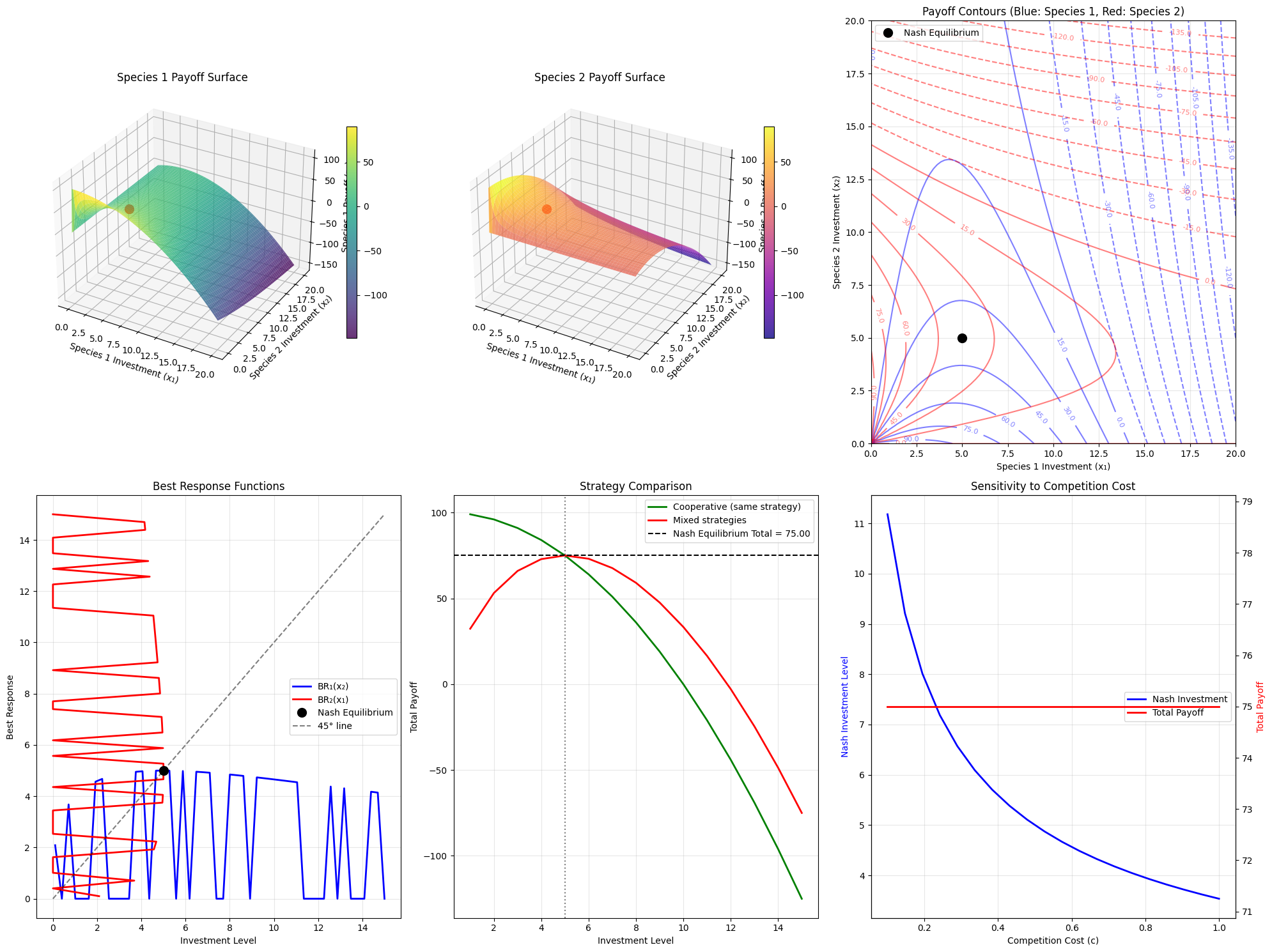
4. Visualization Components
3D Payoff Surfaces: These show how each species’ payoff varies with both investment levels. The red dot marks the Nash equilibrium.
Contour Plots: Provide a 2D view of the payoff landscapes, making it easier to see the strategic interactions.
Best Response Functions: Show how each species should optimally respond to their opponent’s strategy. The intersection point is the Nash equilibrium.
Strategy Comparison: Compares total welfare under different strategic scenarios.
Sensitivity Analysis: Shows how the equilibrium changes with different cost parameters.
Results
Competition Strategy Optimization Results
==================================================
Model Parameters:
  Resource Pool (R): 100
  Competition Cost (c): 0.5

Nash Equilibrium (Numerical): x₁* = 5.000, x₂* = 5.000
Nash Equilibrium (Analytical): x₁* = 5.000, x₂* = 5.000

Equilibrium Payoffs:
  Species 1: π₁* = 37.500
  Species 2: π₂* = 37.500
  Total Payoff: 75.000
Detailed Analysis:
==================================================
At Nash equilibrium, each species invests 5.000 units
This results in each species getting 50.0 units of resource
Total competition investment: 10.000 units
Total cost incurred: 25.000 units
Efficiency loss compared to no competition: 25.000 units
Key Insights from the Results
Strategic Complementarity: The best response functions slope upward, indicating that higher competition from one species incentivizes higher competition from the other.
Inefficiency of Competition: The Nash equilibrium results in both species investing in competition, reducing total welfare compared to a no-competition scenario.
Cost Sensitivity: As competition costs increase, equilibrium investment levels decrease, but total payoffs don’t necessarily increase due to the reduced competitive pressure.
Symmetry: In this symmetric game, both species end up with identical strategies and payoffs at equilibrium.
Mathematical Formulation
The complete mathematical model can be expressed as:
Maximize: $\pi_1(x_1, x_2) = \frac{x_1}{x_1 + x_2} \cdot R - c \cdot x_1^2$
Subject to: $x_1 \geq 0$
Where: Species 2 simultaneously solves the analogous problem
Nash Equilibrium: $(x_1^*, x_2^*) = \left(\sqrt{\frac{R}{8c}}, \sqrt{\frac{R}{8c}}\right)$
This model demonstrates fundamental principles in competition theory and has applications ranging from evolutionary biology to business strategy and economic competition. The key takeaway is that competitive markets often lead to over-investment in competition relative to social optimum, a classic result in game theory known as the “tragedy of competition.”