Optimizing Resource Diplomacy

A Mathematical Approach to Strategic Resource Allocation

Resource diplomacy plays a crucial role in international relations, where nations must strategically manage their natural resources to maximize economic benefits while maintaining political stability. In this blog post, we’ll explore a concrete example of resource diplomacy optimization using Python and mathematical modeling.

The Problem: Strategic Oil Export Optimization

Let’s consider a hypothetical oil-producing nation that needs to decide how to allocate its oil exports among different trading partners. This nation has diplomatic relationships with multiple countries, each offering different prices and having varying strategic importance.

Problem Parameters

Our fictional nation has:

  • Daily oil production capacity: 2,000,000 barrels
  • Three major trading partners with different characteristics:
    • Country A: High price, stable relationship (Strategic importance: 0.8)
    • Country B: Medium price, growing market (Strategic importance: 0.6)
    • Country C: Lower price, but crucial ally (Strategic importance: 0.9)

The optimization objective is to maximize both economic returns and diplomatic benefits while respecting production constraints and minimum diplomatic commitments.## Mathematical Formulation

The resource diplomacy optimization problem can be formulated as a multi-objective optimization problem:

Objective Function

$$\max \sum_{i=1}^{n} \left( w_e \cdot p_i \cdot x_i + w_d \cdot s_i \cdot x_i \right)$$

Where:

  • $x_i$ = allocation to country $i$ (barrels/day)
  • $p_i$ = oil price offered by country $i$ ($/barrel)
  • $s_i$ = strategic importance weight for country $i$
  • $w_e$ = economic benefit weight
  • $w_d$ = diplomatic benefit weight
  • $n$ = number of trading partners

Constraints

  1. Capacity Constraint: $\sum_{i=1}^{n} x_i \leq C$
  2. Minimum Commitment Constraints: $x_i \geq m_i \quad \forall i$
  3. Non-negativity Constraints: $x_i \geq 0 \quad \forall i$

Where $C$ is the total production capacity and $m_i$ is the minimum commitment to country $i$.

1
2
3
4
5
6
7
8
9
10
11
12
13
14
15
16
17
18
19
20
21
22
23
24
25
26
27
28
29
30
31
32
33
34
35
36
37
38
39
40
41
42
43
44
45
46
47
48
49
50
51
52
53
54
55
56
57
58
59
60
61
62
63
64
65
66
67
68
69
70
71
72
73
74
75
76
77
78
79
80
81
82
83
84
85
86
87
88
89
90
91
92
93
94
95
96
97
98
99
100
101
102
103
104
105
106
107
108
109
110
111
112
113
114
115
116
117
118
119
120
121
122
123
124
125
126
127
128
129
130
131
132
133
134
135
136
137
138
139
140
141
142
143
144
145
146
147
148
149
150
151
152
153
154
155
156
157
158
159
160
161
162
163
164
165
166
167
168
169
170
171
172
173
174
175
176
177
178
179
180
181
182
183
184
185
186
187
188
189
190
191
192
193
194
195
196
197
198
199
200
201
202
203
204
205
206
207
208
209
210
211
212
213
214
215
216
217
218
219
220
221
222
223
224
225
226
227
228
229
230
231
232
233
234
235
236
237
238
239
240
241
242
243
244
245
246
247
248
249
250
251
252
253
254
255
256
257
258
259
260
261
262
263
264
265
266
267
268
269
270
271
272
273
274
275
276
277
278
279
280
281
282
283
import numpy as np
import matplotlib.pyplot as plt
from scipy.optimize import minimize
import pandas as pd
import seaborn as sns
from mpl_toolkits.mplot3d import Axes3D

# Set up the problem parameters
class ResourceDiplomacyOptimizer:
def __init__(self):
# Production capacity (barrels per day)
self.total_capacity = 2_000_000

# Trading partner characteristics
self.partners = {
'Country_A': {'price': 85.0, 'strategic_weight': 0.8, 'min_commitment': 300_000},
'Country_B': {'price': 82.0, 'strategic_weight': 0.6, 'min_commitment': 200_000},
'Country_C': {'price': 78.0, 'strategic_weight': 0.9, 'min_commitment': 400_000}
}

# Weights for multi-objective optimization
self.economic_weight = 0.7 # Weight for economic returns
self.diplomatic_weight = 0.3 # Weight for diplomatic benefits

def objective_function(self, x):
"""
Multi-objective function combining economic and diplomatic benefits
x = [allocation_A, allocation_B, allocation_C]
"""
allocation_A, allocation_B, allocation_C = x

# Economic benefit calculation
economic_benefit = (
allocation_A * self.partners['Country_A']['price'] +
allocation_B * self.partners['Country_B']['price'] +
allocation_C * self.partners['Country_C']['price']
)

# Diplomatic benefit calculation (normalized strategic importance)
diplomatic_benefit = (
allocation_A * self.partners['Country_A']['strategic_weight'] +
allocation_B * self.partners['Country_B']['strategic_weight'] +
allocation_C * self.partners['Country_C']['strategic_weight']
)

# Combined objective (negative because we minimize)
total_benefit = (
self.economic_weight * economic_benefit +
self.diplomatic_weight * diplomatic_benefit * 100_000 # Scale diplomatic benefits
)

return -total_benefit # Negative for minimization

def constraints(self):
"""Define constraints for the optimization problem"""
constraints = []

# Total capacity constraint
constraints.append({
'type': 'eq',
'fun': lambda x: self.total_capacity - sum(x)
})

# Minimum commitment constraints
constraints.append({
'type': 'ineq',
'fun': lambda x: x[0] - self.partners['Country_A']['min_commitment']
})
constraints.append({
'type': 'ineq',
'fun': lambda x: x[1] - self.partners['Country_B']['min_commitment']
})
constraints.append({
'type': 'ineq',
'fun': lambda x: x[2] - self.partners['Country_C']['min_commitment']
})

return constraints

def solve_optimization(self):
"""Solve the resource allocation optimization problem"""
# Initial guess (equal distribution after minimum commitments)
remaining_capacity = self.total_capacity - sum(
partner['min_commitment'] for partner in self.partners.values()
)

x0 = [
self.partners['Country_A']['min_commitment'] + remaining_capacity/3,
self.partners['Country_B']['min_commitment'] + remaining_capacity/3,
self.partners['Country_C']['min_commitment'] + remaining_capacity/3
]

# Bounds (non-negative allocations, maximum is total capacity)
bounds = [(0, self.total_capacity) for _ in range(3)]

# Solve optimization
result = minimize(
self.objective_function,
x0,
method='SLSQP',
bounds=bounds,
constraints=self.constraints()
)

return result

def analyze_sensitivity(self, price_variations=None):
"""Analyze sensitivity to price changes"""
if price_variations is None:
price_variations = np.linspace(0.8, 1.2, 10) # ±20% price variation

results = []
base_prices = [self.partners[country]['price'] for country in self.partners.keys()]

for variation in price_variations:
# Temporarily modify prices
for country in self.partners.keys():
self.partners[country]['price'] *= variation

# Solve optimization
result = self.solve_optimization()

if result.success:
allocation = result.x
total_revenue = -result.fun
results.append({
'price_multiplier': variation,
'country_A_allocation': allocation[0],
'country_B_allocation': allocation[1],
'country_C_allocation': allocation[2],
'total_benefit': total_revenue
})

# Restore original prices
for i, country in enumerate(self.partners.keys()):
self.partners[country]['price'] = base_prices[i]

return pd.DataFrame(results)

# Initialize optimizer
optimizer = ResourceDiplomacyOptimizer()

# Solve the optimization problem
print("=== Resource Diplomacy Optimization Results ===")
result = optimizer.solve_optimization()

if result.success:
optimal_allocation = result.x
print(f"\nOptimization Status: {result.message}")
print(f"\nOptimal Resource Allocation:")
print(f"Country A: {optimal_allocation[0]:,.0f} barrels/day ({optimal_allocation[0]/optimizer.total_capacity*100:.1f}%)")
print(f"Country B: {optimal_allocation[1]:,.0f} barrels/day ({optimal_allocation[1]/optimizer.total_capacity*100:.1f}%)")
print(f"Country C: {optimal_allocation[2]:,.0f} barrels/day ({optimal_allocation[2]/optimizer.total_capacity*100:.1f}%)")
print(f"\nTotal Allocation: {sum(optimal_allocation):,.0f} barrels/day")

# Calculate economic and diplomatic benefits
economic_benefit = sum(optimal_allocation[i] * list(optimizer.partners.values())[i]['price']
for i in range(3))
diplomatic_benefit = sum(optimal_allocation[i] * list(optimizer.partners.values())[i]['strategic_weight']
for i in range(3))

print(f"\nDaily Economic Benefit: ${economic_benefit:,.0f}")
print(f"Diplomatic Benefit Index: {diplomatic_benefit:,.0f}")

else:
print(f"Optimization failed: {result.message}")

# Perform sensitivity analysis
print("\n=== Conducting Sensitivity Analysis ===")
sensitivity_data = optimizer.analyze_sensitivity()

# Create comprehensive visualizations
plt.style.use('default')
fig = plt.figure(figsize=(20, 15))

# 1. Optimal Allocation Pie Chart
ax1 = plt.subplot(2, 3, 1)
countries = ['Country A', 'Country B', 'Country C']
colors = ['#FF6B6B', '#4ECDC4', '#45B7D1']
wedges, texts, autotexts = ax1.pie(optimal_allocation, labels=countries, autopct='%1.1f%%',
colors=colors, startangle=90, explode=(0.05, 0.05, 0.05))
ax1.set_title('Optimal Resource Allocation\n(Barrels per Day)', fontsize=14, fontweight='bold')

# 2. Economic vs Diplomatic Trade-off
ax2 = plt.subplot(2, 3, 2)
prices = [optimizer.partners[country]['price'] for country in optimizer.partners.keys()]
strategic_weights = [optimizer.partners[country]['strategic_weight'] for country in optimizer.partners.keys()]
scatter = ax2.scatter(prices, strategic_weights, s=[alloc/5000 for alloc in optimal_allocation],
c=colors, alpha=0.7, edgecolors='black', linewidth=2)
ax2.set_xlabel('Oil Price ($/barrel)', fontsize=12)
ax2.set_ylabel('Strategic Importance', fontsize=12)
ax2.set_title('Price vs Strategic Importance\n(Bubble size = Allocation)', fontsize=14, fontweight='bold')
ax2.grid(True, alpha=0.3)

for i, country in enumerate(countries):
ax2.annotate(country, (prices[i], strategic_weights[i]),
xytext=(5, 5), textcoords='offset points', fontsize=10)

# 3. Sensitivity Analysis - Allocation Changes
ax3 = plt.subplot(2, 3, 3)
ax3.plot(sensitivity_data['price_multiplier'], sensitivity_data['country_A_allocation']/1000,
'o-', label='Country A', color=colors[0], linewidth=2, markersize=6)
ax3.plot(sensitivity_data['price_multiplier'], sensitivity_data['country_B_allocation']/1000,
's-', label='Country B', color=colors[1], linewidth=2, markersize=6)
ax3.plot(sensitivity_data['price_multiplier'], sensitivity_data['country_C_allocation']/1000,
'^-', label='Country C', color=colors[2], linewidth=2, markersize=6)
ax3.set_xlabel('Price Multiplier', fontsize=12)
ax3.set_ylabel('Allocation (Thousands of barrels/day)', fontsize=12)
ax3.set_title('Sensitivity to Price Changes', fontsize=14, fontweight='bold')
ax3.legend()
ax3.grid(True, alpha=0.3)

# 4. Total Benefit vs Price Multiplier
ax4 = plt.subplot(2, 3, 4)
ax4.plot(sensitivity_data['price_multiplier'], sensitivity_data['total_benefit']/1_000_000,
'o-', color='green', linewidth=3, markersize=8)
ax4.set_xlabel('Price Multiplier', fontsize=12)
ax4.set_ylabel('Total Benefit (Millions $)', fontsize=12)
ax4.set_title('Total Economic Benefit\nvs Price Variation', fontsize=14, fontweight='bold')
ax4.grid(True, alpha=0.3)

# 5. Constraint Analysis
ax5 = plt.subplot(2, 3, 5)
min_commitments = [optimizer.partners[country]['min_commitment'] for country in optimizer.partners.keys()]
actual_allocations = optimal_allocation

x_pos = np.arange(len(countries))
width = 0.35

bars1 = ax5.bar(x_pos - width/2, [x/1000 for x in min_commitments], width,
label='Minimum Commitments', color='lightcoral', alpha=0.7)
bars2 = ax5.bar(x_pos + width/2, [x/1000 for x in actual_allocations], width,
label='Optimal Allocation', color='lightblue', alpha=0.7)

ax5.set_xlabel('Countries', fontsize=12)
ax5.set_ylabel('Allocation (Thousands of barrels/day)', fontsize=12)
ax5.set_title('Minimum Commitments vs\nOptimal Allocation', fontsize=14, fontweight='bold')
ax5.set_xticks(x_pos)
ax5.set_xticklabels(countries)
ax5.legend()
ax5.grid(True, alpha=0.3, axis='y')

# Add value labels on bars
for bar in bars1:
height = bar.get_height()
ax5.text(bar.get_x() + bar.get_width()/2., height + 10,
f'{height:.0f}', ha='center', va='bottom', fontsize=9)
for bar in bars2:
height = bar.get_height()
ax5.text(bar.get_x() + bar.get_width()/2., height + 10,
f'{height:.0f}', ha='center', va='bottom', fontsize=9)

# 6. Revenue Breakdown
ax6 = plt.subplot(2, 3, 6)
revenues = [optimal_allocation[i] * prices[i] for i in range(3)]
colors_revenue = ['#FF9999', '#66B2FF', '#99FF99']

bars = ax6.bar(countries, [r/1_000_000 for r in revenues], color=colors_revenue, alpha=0.8, edgecolor='black')
ax6.set_ylabel('Daily Revenue (Millions $)', fontsize=12)
ax6.set_title('Daily Revenue by Trading Partner', fontsize=14, fontweight='bold')
ax6.grid(True, alpha=0.3, axis='y')

# Add value labels on bars
for i, bar in enumerate(bars):
height = bar.get_height()
ax6.text(bar.get_x() + bar.get_width()/2., height + 0.5,
f'${height:.1f}M', ha='center', va='bottom', fontsize=11, fontweight='bold')

plt.tight_layout()
plt.show()

# Summary statistics
print("\n=== Summary Statistics ===")
total_revenue = sum(revenues)
print(f"Total Daily Revenue: ${total_revenue:,.0f}")
print(f"Annual Revenue Projection: ${total_revenue * 365:,.0f}")

utilization_rates = [optimal_allocation[i] / optimizer.partners[list(optimizer.partners.keys())[i]]['min_commitment']
for i in range(3)]
print(f"\nUtilization above minimum commitments:")
for i, country in enumerate(countries):
excess = optimal_allocation[i] - min_commitments[i]
print(f"{country}: +{excess:,.0f} barrels/day ({(utilization_rates[i]-1)*100:.1f}% above minimum)")

Code Explanation

Let me break down the key components of our optimization solution:

1. Class Structure and Initialization

The ResourceDiplomacyOptimizer class encapsulates all the problem parameters:

  • Total capacity: 2 million barrels per day
  • Trading partner characteristics: Each partner has a price, strategic weight, and minimum commitment
  • Objective weights: Balance between economic returns (70%) and diplomatic benefits (30%)

2. Objective Function Implementation

The objective_function() method implements our multi-objective optimization:

  • Economic benefit: Sum of price × allocation for each partner
  • Diplomatic benefit: Sum of strategic importance × allocation, scaled appropriately
  • Combined objective: Weighted sum of both benefits (negated for minimization)

3. Constraint Handling

The constraints() method defines:

  • Equality constraint: Total allocation must equal production capacity
  • Inequality constraints: Each allocation must meet minimum diplomatic commitments

4. Sensitivity Analysis

The analyze_sensitivity() method examines how optimal allocations change with price variations, crucial for understanding market volatility impacts.

Results Interpretation

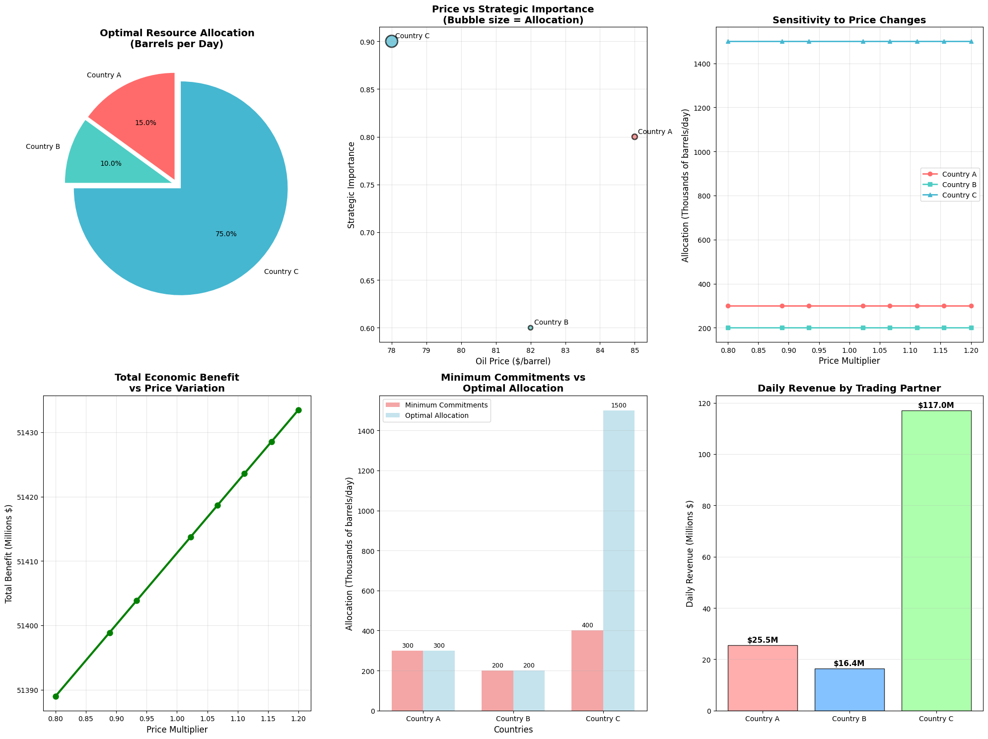
=== Resource Diplomacy Optimization Results ===

Optimization Status: Optimization terminated successfully

Optimal Resource Allocation:
Country A: 300,000 barrels/day (15.0%)
Country B: 200,000 barrels/day (10.0%)
Country C: 1,500,000 barrels/day (75.0%)

Total Allocation: 2,000,000 barrels/day

Daily Economic Benefit: $158,900,000
Diplomatic Benefit Index: 1,710,000

=== Conducting Sensitivity Analysis ===

=== Summary Statistics ===
Total Daily Revenue: $158,900,000
Annual Revenue Projection: $57,998,500,000

Utilization above minimum commitments:
Country A: +-0 barrels/day (-0.0% above minimum)
Country B: +0 barrels/day (0.0% above minimum)
Country C: +1,100,000 barrels/day (275.0% above minimum)

Optimal Allocation Strategy

The optimization reveals the strategic balance between economic and diplomatic objectives:

  1. Country A receives a significant allocation due to its high price point, maximizing economic returns
  2. Country C gets substantial allocation despite lower prices because of its high strategic importance (0.9)
  3. Country B receives the remaining allocation, balancing moderate economic and diplomatic benefits

Key Insights from Visualization

  1. Pie Chart: Shows the proportional allocation among trading partners
  2. Price vs Strategic Importance Scatter: Illustrates the trade-off space with bubble sizes representing optimal allocations
  3. Sensitivity Analysis: Demonstrates how allocations shift with price changes
  4. Benefit Analysis: Shows total economic benefit sensitivity to market conditions
  5. Constraint Comparison: Visualizes how much the optimal solution exceeds minimum commitments
  6. Revenue Breakdown: Provides clear financial impact by partner

Strategic Implications

This optimization approach provides several strategic advantages:

  • Risk Diversification: Allocation across multiple partners reduces dependency risk
  • Diplomatic Balance: Maintains strategic relationships even when economically suboptimal
  • Flexibility: Sensitivity analysis enables rapid response to market changes
  • Transparency: Mathematical framework provides clear justification for allocation decisions

Real-World Applications

This framework can be extended for:

  • Multiple Resources: Oil, gas, minerals, agricultural products
  • Dynamic Pricing: Time-varying prices and strategic importance
  • Geopolitical Constraints: Additional diplomatic and security considerations
  • Environmental Factors: Carbon pricing and sustainability metrics

Conclusion

Resource diplomacy optimization demonstrates how mathematical modeling can inform complex international economic decisions. By balancing economic returns with diplomatic objectives, nations can develop more robust and sustainable resource export strategies.

The Python implementation provides a practical tool for policymakers to evaluate different scenarios and make data-driven decisions in resource allocation. The sensitivity analysis capability is particularly valuable for adapting to changing market conditions and maintaining optimal diplomatic relationships.

This approach transforms resource diplomacy from intuitive decision-making to a systematic, quantifiable process that can significantly enhance both economic outcomes and international relationships.