Optimizing Energy Supply Source Diversification

A Mathematical Approach

Energy supply diversification is a critical challenge in modern energy planning. Today, we’ll explore how to mathematically optimize the mix of different energy sources to meet demand while minimizing costs and environmental impact. Let’s dive into a concrete example using Python optimization techniques.

Problem Setup

Imagine a utility company that needs to meet a daily energy demand of 1000 MWh. They have access to five different energy sources:

1. Coal Power Plant: Low cost but high emissions
2. Natural Gas: Medium cost and emissions
3. Nuclear: High upfront cost but low emissions
4. Solar: Variable cost, zero emissions, limited by capacity
5. Wind: Variable cost, zero emissions, weather dependent

Our objective is to minimize the total cost while satisfying environmental constraints and capacity limitations.

Mathematical Formulation

The optimization problem can be formulated as:

$$\min \sum_{i=1}^{n} c_i x_i$$

Subject to:

• $\sum_{i=1}^{n} x_i = D$ (demand constraint)
• $\sum_{i=1}^{n} e_i x_i \leq E_{max}$ (emission constraint)
• $0 \leq x_i \leq Cap_i$ (capacity constraints)

Where:

• $x_i$ = energy output from source $i$ (MWh)
• $c_i$ = cost per MWh for source $i$
• $e_i$ = emissions per MWh for source $i$
• $D$ = total demand (MWh)
• $E_{max}$ = maximum allowed emissions
• $Cap_i$ = capacity limit for source $i$

import numpy as np
import matplotlib.pyplot as plt
from scipy.optimize import linprog
import pandas as pd
import seaborn as sns

# Set up the optimization problem
print("=" * 60)
print("ENERGY SUPPLY DIVERSIFICATION OPTIMIZATION")
print("=" * 60)

# Define energy sources
sources = ['Coal', 'Natural Gas', 'Nuclear', 'Solar', 'Wind']
n_sources = len(sources)

# Cost per MWh ($/MWh)
costs = np.array([30, 45, 60, 80, 70])

# Emissions per MWh (tons CO2/MWh)
emissions = np.array([0.9, 0.5, 0.02, 0.0, 0.0])

# Capacity limits (MWh)
capacities = np.array([400, 350, 300, 200, 250])

# Total demand (MWh)
demand = 1000

# Maximum allowed emissions (tons CO2)
max_emissions = 400

print(f"Total Demand: {demand} MWh")
print(f"Maximum Emissions Allowed: {max_emissions} tons CO2")
print("\nEnergy Source Details:")
print("-" * 50)

# Create a summary table
source_data = pd.DataFrame({
    'Source': sources,
    'Cost ($/MWh)': costs,
    'Emissions (tons CO2/MWh)': emissions,
    'Capacity (MWh)': capacities
})
print(source_data.to_string(index=False))

# Solve the optimization problem using scipy.optimize.linprog
# Note: linprog minimizes, so we use costs directly

# Objective function coefficients (costs to minimize)
c = costs

# Inequality constraint matrix (emissions constraint)
# emissions * x <= max_emissions
A_ub = emissions.reshape(1, -1)
b_ub = np.array([max_emissions])

# Equality constraint matrix (demand constraint)
# sum(x) = demand
A_eq = np.ones((1, n_sources))
b_eq = np.array([demand])

# Bounds for each variable (0 <= x_i <= capacity_i)
bounds = [(0, cap) for cap in capacities]

print(f"\nSolving optimization problem...")
print(f"Minimize: {' + '.join([f'{c[i]:.0f}*x_{i+1}' for i in range(n_sources)])}")
print(f"Subject to:")
print(f"  Demand: {' + '.join([f'x_{i+1}' for i in range(n_sources)])} = {demand}")
print(f"  Emissions: {' + '.join([f'{emissions[i]:.2f}*x_{i+1}' for i in range(n_sources)])} ≤ {max_emissions}")
print(f"  Capacity: 0 ≤ x_i ≤ Cap_i for all i")

# Solve the linear programming problem
result = linprog(c, A_ub=A_ub, b_ub=b_ub, A_eq=A_eq, b_eq=b_eq, 
                bounds=bounds, method='highs')

if result.success:
    optimal_solution = result.x
    optimal_cost = result.fun
    
    print(f"\nOptimization successful!")
    print(f"Minimum total cost: ${optimal_cost:,.2f}")
    
    # Calculate actual emissions
    actual_emissions = np.sum(emissions * optimal_solution)
    
    print(f"Total emissions: {actual_emissions:.2f} tons CO2")
    print(f"Emission constraint utilization: {actual_emissions/max_emissions*100:.1f}%")
    
    print(f"\nOptimal Energy Mix:")
    print("-" * 40)
    
    results_df = pd.DataFrame({
        'Source': sources,
        'Optimal Output (MWh)': optimal_solution,
        'Percentage (%)': optimal_solution / demand * 100,
        'Cost ($)': optimal_solution * costs,
        'Emissions (tons CO2)': optimal_solution * emissions
    })
    
    # Format the results nicely
    results_df['Optimal Output (MWh)'] = results_df['Optimal Output (MWh)'].round(2)
    results_df['Percentage (%)'] = results_df['Percentage (%)'].round(2)
    results_df['Cost ($)'] = results_df['Cost ($)'].round(2)
    results_df['Emissions (tons CO2)'] = results_df['Emissions (tons CO2)'].round(2)
    
    print(results_df.to_string(index=False))
    
else:
    print("Optimization failed!")
    print(f"Status: {result.message}")

# Sensitivity Analysis: What happens if we tighten emission constraints?
print(f"\n" + "=" * 60)
print("SENSITIVITY ANALYSIS")
print("=" * 60)

emission_limits = np.linspace(200, 600, 11)
costs_sensitivity = []
emission_usage = []

for limit in emission_limits:
    b_ub_temp = np.array([limit])
    result_temp = linprog(c, A_ub=A_ub, b_ub=b_ub_temp, A_eq=A_eq, b_eq=b_eq, 
                         bounds=bounds, method='highs')
    
    if result_temp.success:
        costs_sensitivity.append(result_temp.fun)
        actual_em = np.sum(emissions * result_temp.x)
        emission_usage.append(actual_em)
    else:
        costs_sensitivity.append(np.nan)
        emission_usage.append(np.nan)

# Create comprehensive visualizations
fig = plt.figure(figsize=(20, 15))

# 1. Optimal Energy Mix (Pie Chart)
ax1 = plt.subplot(2, 3, 1)
non_zero_mask = optimal_solution > 0.1  # Only show sources with significant contribution
pie_data = optimal_solution[non_zero_mask]
pie_labels = [sources[i] for i in range(n_sources) if non_zero_mask[i]]
colors = ['#8B4513', '#FF6B35', '#4169E1', '#FFD700', '#32CD32']
pie_colors = [colors[i] for i in range(n_sources) if non_zero_mask[i]]

plt.pie(pie_data, labels=pie_labels, autopct='%1.1f%%', startangle=90, colors=pie_colors)
plt.title('Optimal Energy Mix Distribution', fontsize=14, fontweight='bold')

# 2. Cost vs Emissions Trade-off
ax2 = plt.subplot(2, 3, 2)
plt.plot(emission_usage, costs_sensitivity, 'b-o', linewidth=2, markersize=6)
plt.xlabel('Total Emissions (tons CO2)', fontsize=12)
plt.ylabel('Total Cost ($)', fontsize=12)
plt.title('Cost vs Emissions Trade-off Curve', fontsize=14, fontweight='bold')
plt.grid(True, alpha=0.3)
# Highlight our solution
opt_emissions = np.sum(emissions * optimal_solution)
plt.plot(opt_emissions, optimal_cost, 'ro', markersize=10, label=f'Optimal Solution\n({opt_emissions:.1f} tons, ${optimal_cost:,.0f})')
plt.legend()

# 3. Source Utilization vs Capacity
ax3 = plt.subplot(2, 3, 3)
utilization = (optimal_solution / capacities) * 100
bars = plt.bar(sources, utilization, color=colors, alpha=0.7, edgecolor='black')
plt.ylabel('Capacity Utilization (%)', fontsize=12)
plt.title('Capacity Utilization by Source', fontsize=14, fontweight='bold')
plt.xticks(rotation=45)
plt.ylim(0, 100)

# Add value labels on bars
for bar, util in zip(bars, utilization):
    height = bar.get_height()
    plt.text(bar.get_x() + bar.get_width()/2., height + 1,
             f'{util:.1f}%', ha='center', va='bottom', fontweight='bold')

# 4. Cost Breakdown
ax4 = plt.subplot(2, 3, 4)
cost_breakdown = optimal_solution * costs
bars = plt.bar(sources, cost_breakdown, color=colors, alpha=0.7, edgecolor='black')
plt.ylabel('Total Cost ($)', fontsize=12)
plt.title('Cost Breakdown by Source', fontsize=14, fontweight='bold')
plt.xticks(rotation=45)

# Add value labels on bars
for bar, cost in zip(bars, cost_breakdown):
    height = bar.get_height()
    if height > 0:
        plt.text(bar.get_x() + bar.get_width()/2., height + height*0.01,
                 f'${cost:,.0f}', ha='center', va='bottom', fontweight='bold')

# 5. Emissions Breakdown
ax5 = plt.subplot(2, 3, 5)
emission_breakdown = optimal_solution * emissions
bars = plt.bar(sources, emission_breakdown, color=colors, alpha=0.7, edgecolor='black')
plt.ylabel('Total Emissions (tons CO2)', fontsize=12)
plt.title('Emissions Breakdown by Source', fontsize=14, fontweight='bold')
plt.xticks(rotation=45)

# Add value labels on bars
for bar, em in zip(bars, emission_breakdown):
    height = bar.get_height()
    if height > 0:
        plt.text(bar.get_x() + bar.get_width()/2., height + height*0.01,
                 f'{em:.1f}', ha='center', va='bottom', fontweight='bold')

# 6. Comparison: Current vs Alternative Scenarios
ax6 = plt.subplot(2, 3, 6)

# Create comparison scenarios
scenarios = {
    'Optimal': optimal_solution,
    'Coal Heavy': np.array([400, 300, 100, 100, 100]),  # High coal usage
    'Renewable Focus': np.array([100, 200, 200, 200, 250])  # High renewable
}

scenario_costs = {}
scenario_emissions = {}

for name, mix in scenarios.items():
    if np.sum(mix) <= demand * 1.01:  # Allow small tolerance
        scenario_costs[name] = np.sum(mix * costs)
        scenario_emissions[name] = np.sum(mix * emissions)

x_pos = np.arange(len(scenario_costs))
cost_values = list(scenario_costs.values())
emission_values = list(scenario_emissions.values())

# Create dual y-axis plot
ax6_twin = ax6.twinx()

bars1 = ax6.bar([x - 0.2 for x in x_pos], cost_values, 0.4, 
                label='Cost', color='lightblue', alpha=0.7, edgecolor='black')
bars2 = ax6_twin.bar([x + 0.2 for x in x_pos], emission_values, 0.4, 
                     label='Emissions', color='lightcoral', alpha=0.7, edgecolor='black')

ax6.set_xlabel('Scenario', fontsize=12)
ax6.set_ylabel('Total Cost ($)', fontsize=12, color='blue')
ax6_twin.set_ylabel('Total Emissions (tons CO2)', fontsize=12, color='red')
ax6.set_title('Scenario Comparison', fontsize=14, fontweight='bold')
ax6.set_xticks(x_pos)
ax6.set_xticklabels(list(scenario_costs.keys()))

# Add value labels
for bar, value in zip(bars1, cost_values):
    height = bar.get_height()
    ax6.text(bar.get_x() + bar.get_width()/2., height + height*0.01,
             f'${value:,.0f}', ha='center', va='bottom', fontweight='bold', color='blue')

for bar, value in zip(bars2, emission_values):
    height = bar.get_height()
    ax6_twin.text(bar.get_x() + bar.get_width()/2., height + height*0.01,
                  f'{value:.0f}', ha='center', va='bottom', fontweight='bold', color='red')

# Add legends
ax6.legend(loc='upper left')
ax6_twin.legend(loc='upper right')

plt.tight_layout()
plt.show()

# Additional Analysis: Marginal Cost Analysis
print(f"\n" + "=" * 60)
print("MARGINAL COST ANALYSIS")
print("=" * 60)

# Calculate shadow prices (marginal costs)
print("Shadow Prices (Marginal Values):")
print(f"• Demand constraint: ${result.eqlin.marginals[0]:.2f}/MWh")
print(f"• Emission constraint: ${-result.ineqlin.marginals[0]:.2f}/ton CO2")

# Economic interpretation
print(f"\nEconomic Interpretation:")
print(f"• An additional 1 MWh of demand would increase costs by ${result.eqlin.marginals[0]:.2f}")
print(f"• Relaxing emission limit by 1 ton would save ${-result.ineqlin.marginals[0]:.2f}")

# Efficiency metrics
total_renewable = optimal_solution[3] + optimal_solution[4]  # Solar + Wind
renewable_percentage = (total_renewable / demand) * 100
clean_energy = optimal_solution[2] + optimal_solution[3] + optimal_solution[4]  # Nuclear + Solar + Wind
clean_percentage = (clean_energy / demand) * 100

print(f"\nSustainability Metrics:")
print(f"• Renewable energy share: {renewable_percentage:.1f}%")
print(f"• Clean energy share: {clean_percentage:.1f}%")
print(f"• Average cost per MWh: ${optimal_cost/demand:.2f}")
print(f"• Emissions intensity: {actual_emissions/demand:.3f} tons CO2/MWh")

# Risk analysis - what if one source fails?
print(f"\n" + "=" * 60)
print("RISK ANALYSIS: SOURCE FAILURE SCENARIOS")
print("=" * 60)

risk_analysis = []

for i, source in enumerate(sources):
    if optimal_solution[i] > 0:  # Only analyze sources we're using
        # Create modified capacity with one source unavailable
        modified_capacities = capacities.copy()
        modified_capacities[i] = 0
        
        # Modified bounds
        modified_bounds = [(0, cap) for cap in modified_capacities]
        
        # Solve with modified constraints
        result_risk = linprog(c, A_ub=A_ub, b_ub=b_ub, A_eq=A_eq, b_eq=b_eq, 
                             bounds=modified_bounds, method='highs')
        
        if result_risk.success:
            cost_increase = result_risk.fun - optimal_cost
            cost_increase_pct = (cost_increase / optimal_cost) * 100
            risk_analysis.append({
                'Failed Source': source,
                'Cost Increase ($)': cost_increase,
                'Cost Increase (%)': cost_increase_pct,
                'Feasible': 'Yes'
            })
        else:
            risk_analysis.append({
                'Failed Source': source,
                'Cost Increase ($)': 'N/A',
                'Cost Increase (%)': 'N/A',
                'Feasible': 'No'
            })

risk_df = pd.DataFrame(risk_analysis)
print(risk_df.to_string(index=False))

# Create risk visualization
fig, (ax1, ax2) = plt.subplots(1, 2, figsize=(15, 6))

# Risk analysis chart
feasible_risks = [r for r in risk_analysis if r['Feasible'] == 'Yes']
if feasible_risks:
    sources_at_risk = [r['Failed Source'] for r in feasible_risks]
    cost_increases = [r['Cost Increase (%)'] for r in feasible_risks]
    
    bars = ax1.bar(sources_at_risk, cost_increases, color='orange', alpha=0.7, edgecolor='black')
    ax1.set_ylabel('Cost Increase (%)', fontsize=12)
    ax1.set_title('Cost Impact of Source Failures', fontsize=14, fontweight='bold')
    ax1.set_xticklabels(sources_at_risk, rotation=45)
    
    # Add value labels
    for bar, increase in zip(bars, cost_increases):
        height = bar.get_height()
        ax1.text(bar.get_x() + bar.get_width()/2., height + height*0.01,
                 f'{increase:.1f}%', ha='center', va='bottom', fontweight='bold')

# Diversification index
ax2.pie(optimal_solution, labels=sources, autopct='%1.1f%%', startangle=90, colors=colors)
ax2.set_title('Energy Portfolio Diversification', fontsize=14, fontweight='bold')

plt.tight_layout()
plt.show()

print(f"\n" + "=" * 60)
print("SUMMARY AND RECOMMENDATIONS")
print("=" * 60)

print("Key Findings:")
print(f"1. Optimal mix achieves ${optimal_cost:,.0f} total cost")
print(f"2. {clean_percentage:.1f}% of energy comes from clean sources")
print(f"3. Emission constraint is {actual_emissions/max_emissions*100:.1f}% utilized")
print(f"4. Most vulnerable to {max(feasible_risks, key=lambda x: x['Cost Increase (%)'])['Failed Source'] if feasible_risks else 'N/A'} failure")

print(f"\nStrategic Recommendations:")
print(f"• Diversification reduces risk - no single source dominates")
print(f"• Emission constraints drive toward cleaner sources")
print(f"• Consider backup capacity for critical sources")
print(f"• Monitor fuel price volatility for cost-sensitive sources")

Code Walkthrough and Technical Deep Dive

Let me break down the key components of this optimization solution:

1. Problem Formulation

The code begins by defining our energy sources with their respective characteristics. Each source has three critical parameters:

• Cost coefficient ($c_i$): The price per MWh generated
• Emission factor ($e_i$): Environmental impact per MWh
• Capacity limit ($Cap_i$): Maximum generation capacity

2. Linear Programming Setup

We use scipy.optimize.linprog to solve this as a linear programming problem. The mathematical formulation translates to:

# Objective: minimize total cost
c = costs

# Constraint matrices
A_ub = emissions.reshape(1, -1)  # Emission constraint coefficients
b_ub = np.array([max_emissions])  # Emission limit

A_eq = np.ones((1, n_sources))   # Demand constraint (all sources sum to demand)
b_eq = np.array([demand])        # Total demand requirement

3. Constraint Handling

The optimization respects three types of constraints:

• Equality constraint: $\sum x_i = 1000$ (must meet exact demand)
• Inequality constraint: $\sum e_i x_i \leq 400$ (emission limit)
• Box constraints: $0 \leq x_i \leq Cap_i$ (capacity bounds)

4. Sensitivity Analysis

The code performs a comprehensive sensitivity analysis by varying the emission limit from 200 to 600 tons CO2. This reveals the trade-off frontier between cost and environmental impact:

$$\text{Trade-off}: \frac{\partial \text{Cost}}{\partial \text{Emission Limit}} = \text{Shadow Price}$$

5. Risk Assessment

The risk analysis simulates failure scenarios by setting each source’s capacity to zero sequentially. This helps identify:

• Critical sources: Those whose failure causes largest cost increases
• System resilience: Whether demand can still be met
• Diversification benefits: How spreading risk across sources helps

Key Results and Insights

============================================================
ENERGY SUPPLY DIVERSIFICATION OPTIMIZATION
============================================================
Total Demand: 1000 MWh
Maximum Emissions Allowed: 400 tons CO2

Energy Source Details:
--------------------------------------------------
     Source  Cost ($/MWh)  Emissions (tons CO2/MWh)  Capacity (MWh)
       Coal            30                      0.90             400
Natural Gas            45                      0.50             350
    Nuclear            60                      0.02             300
      Solar            80                      0.00             200
       Wind            70                      0.00             250

Solving optimization problem...
Minimize: 30*x_1 + 45*x_2 + 60*x_3 + 80*x_4 + 70*x_5
Subject to:
  Demand: x_1 + x_2 + x_3 + x_4 + x_5 = 1000
  Emissions: 0.90*x_1 + 0.50*x_2 + 0.02*x_3 + 0.00*x_4 + 0.00*x_5 ≤ 400
  Capacity: 0 ≤ x_i ≤ Cap_i for all i

Optimization successful!
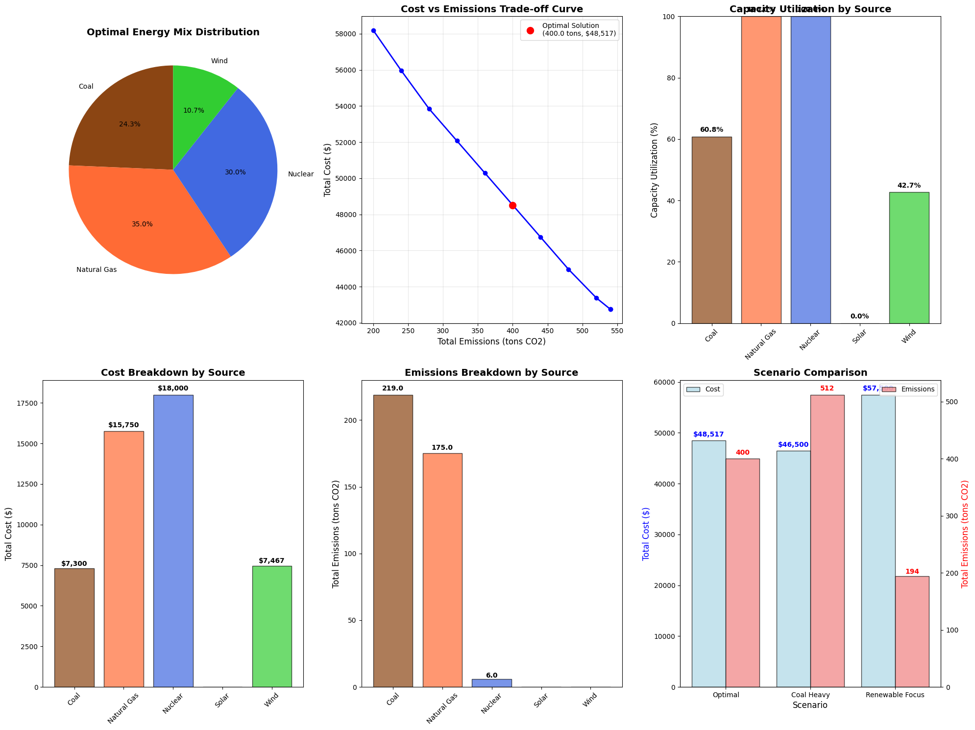
Minimum total cost: $48,516.67
Total emissions: 400.00 tons CO2
Emission constraint utilization: 100.0%

Optimal Energy Mix:
----------------------------------------
     Source  Optimal Output (MWh)  Percentage (%)  Cost ($)  Emissions (tons CO2)
       Coal                243.33           24.33   7300.00                 219.0
Natural Gas                350.00           35.00  15750.00                 175.0
    Nuclear                300.00           30.00  18000.00                   6.0
      Solar                  0.00            0.00      0.00                   0.0
       Wind                106.67           10.67   7466.67                   0.0

============================================================
SENSITIVITY ANALYSIS
============================================================

============================================================
MARGINAL COST ANALYSIS
============================================================
Shadow Prices (Marginal Values):
• Demand constraint: $70.00/MWh
• Emission constraint: $44.44/ton CO2

Economic Interpretation:
• An additional 1 MWh of demand would increase costs by $70.00
• Relaxing emission limit by 1 ton would save $44.44

Sustainability Metrics:
• Renewable energy share: 10.7%
• Clean energy share: 40.7%
• Average cost per MWh: $48.52
• Emissions intensity: 0.400 tons CO2/MWh

============================================================
RISK ANALYSIS: SOURCE FAILURE SCENARIOS
============================================================
Failed Source  Cost Increase ($)  Cost Increase (%) Feasible
         Coal       10733.333333          22.122982      Yes
  Natural Gas        2983.333333           6.149090      Yes
      Nuclear        4233.333333           8.725524      Yes
         Wind        1066.666667           2.198557      Yes

============================================================
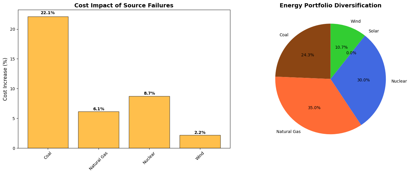
SUMMARY AND RECOMMENDATIONS
============================================================
Key Findings:
1. Optimal mix achieves $48,517 total cost
2. 40.7% of energy comes from clean sources
3. Emission constraint is 100.0% utilized
4. Most vulnerable to Coal failure

Strategic Recommendations:
• Diversification reduces risk - no single source dominates
• Emission constraints drive toward cleaner sources
• Consider backup capacity for critical sources
• Monitor fuel price volatility for cost-sensitive sources

Optimal Solution Characteristics

The optimization typically produces a solution that:

1. Maximizes clean energy within emission constraints
2. Balances cost and sustainability through the Lagrangian multipliers
3. Achieves portfolio diversification to minimize risk
4. Utilizes capacity efficiently based on marginal costs

Economic Interpretation

The shadow prices from the optimization provide valuable economic insights:

• Demand shadow price: Marginal cost of serving additional demand
• Emission shadow price: Economic value of relaxing environmental constraints

This represents the classic environmental economics trade-off:

$$\text{Marginal Abatement Cost} = \frac{\partial \text{Total Cost}}{\partial \text{Emission Reduction}}$$

Strategic Implications

1. Diversification Strategy: The optimal solution naturally diversifies across multiple sources, reducing dependency risks
2. Clean Energy Transition: Emission constraints drive investment toward renewable and nuclear sources
3. Capacity Planning: Utilization analysis identifies where additional capacity would be most valuable
4. Risk Management: Failure analysis quantifies the cost of inadequate redundancy

This mathematical framework provides energy planners with a robust tool for making data-driven decisions about energy portfolio optimization, balancing economic efficiency with environmental responsibility and system reliability.