Optimizing Atomic Traps

A Deep Dive into Magneto-Optical Trap Parameters

Atomic trapping is one of the most fascinating areas of modern physics, enabling us to cool and confine atoms to temperatures near absolute zero. Today, we’ll explore the optimization of a Magneto-Optical Trap (MOT) using Python, focusing on how different parameters affect trapping efficiency.

The Physics Behind Atomic Trapping

A Magneto-Optical Trap combines laser cooling with magnetic confinement. The key physics involves:

  • Doppler cooling: Using laser light slightly red-detuned from an atomic transition
  • Magnetic gradient: Creating a spatially varying magnetic field
  • Scattering force: The momentum transfer from photon absorption/emission

The scattering force on an atom can be expressed as:

F=kΓs01+s0+(2δ/Γ)2

Where:

  • k is the photon momentum
  • Γ is the natural linewidth
  • s0 is the saturation parameter
  • δ is the detuning from resonance

Our Optimization Problem

Let’s consider optimizing a MOT for Rubidium-87 atoms. We’ll maximize the number of trapped atoms by optimizing:

  1. Laser detuning (δ)
  2. Laser intensity (saturation parameter s0)
  3. Magnetic field gradient
1
2
3
4
5
6
7
8
9
10
11
12
13
14
15
16
17
18
19
20
21
22
23
24
25
26
27
28
29
30
31
32
33
34
35
36
37
38
39
40
41
42
43
44
45
46
47
48
49
50
51
52
53
54
55
56
57
58
59
60
61
62
63
64
65
66
67
68
69
70
71
72
73
74
75
76
77
78
79
80
81
82
83
84
85
86
87
88
89
90
91
92
93
94
95
96
97
98
99
100
101
102
103
104
105
106
107
108
109
110
111
112
113
114
115
116
117
118
119
120
121
122
123
124
125
126
127
128
129
130
131
132
133
134
135
136
137
138
139
140
141
142
143
144
145
146
147
148
149
150
151
152
153
154
155
156
157
158
159
160
161
162
163
164
165
166
167
168
169
170
171
172
173
174
175
176
177
178
179
180
181
182
183
184
185
186
187
188
189
190
191
192
193
194
195
196
197
198
199
200
201
202
203
204
205
206
207
208
209
210
211
212
213
214
215
216
217
218
219
220
221
222
223
224
225
226
227
228
229
230
231
232
233
234
235
236
237
238
239
240
241
242
243
244
245
246
247
248
249
250
251
252
253
254
255
256
257
258
259
260
261
262
263
264
265
266
267
268
269
270
271
272
273
274
275
276
277
278
279
280
281
282
283
284
285
286
287
import numpy as np
import matplotlib.pyplot as plt
from scipy.optimize import minimize
from mpl_toolkits.mplot3d import Axes3D

# Physical constants for Rb-87
class Rb87Constants:
def __init__(self):
self.Gamma = 2 * np.pi * 6.067e6 # Natural linewidth (rad/s)
self.lambda_laser = 780.241e-9 # Transition wavelength (m)
self.k = 2 * np.pi / self.lambda_laser # Wave vector
self.mass = 1.443e-25 # Mass of Rb-87 (kg)
self.mu_B = 9.274e-24 # Bohr magneton (J/T)
self.g_J = 2.0 # Landé g-factor
self.hbar = 1.055e-34 # Reduced Planck constant

# Initialize constants
rb87 = Rb87Constants()

class MOTSimulation:
def __init__(self, constants):
self.const = constants

def scattering_rate(self, detuning, saturation_param):
"""
Calculate photon scattering rate

Parameters:
detuning: Laser detuning from resonance (Hz)
saturation_param: Saturation parameter s0

Returns:
Scattering rate (photons/s)
"""
delta_normalized = 2 * detuning / self.const.Gamma
rate = self.const.Gamma * saturation_param / (1 + saturation_param + delta_normalized**2)
return rate

def radiation_pressure_force(self, velocity, detuning, saturation_param, magnetic_gradient, position):
"""
Calculate the total radiation pressure force on an atom

Parameters:
velocity: Atomic velocity (m/s)
detuning: Base laser detuning (Hz)
saturation_param: Saturation parameter
magnetic_gradient: Magnetic field gradient (T/m)
position: Atomic position (m)

Returns:
Force (N)
"""
# Doppler shift
doppler_shift = self.const.k * velocity

# Zeeman shift due to magnetic field
zeeman_shift = self.const.mu_B * self.const.g_J * magnetic_gradient * position / self.const.hbar

# Effective detuning
eff_detuning = detuning + doppler_shift - zeeman_shift

# Scattering rate
scatter_rate = self.scattering_rate(eff_detuning, saturation_param)

# Force (assuming counter-propagating beams)
force = -self.const.hbar * self.const.k * scatter_rate * np.sign(velocity)

return force

def capture_velocity(self, detuning, saturation_param, magnetic_gradient):
"""
Calculate maximum capture velocity for the MOT
"""
# Simplified model: maximum velocity that can be slowed to zero
max_accel = abs(self.radiation_pressure_force(100, detuning, saturation_param, magnetic_gradient, 0.001))
capture_distance = 0.01 # 1 cm typical MOT size

# Using v^2 = 2*a*d
v_capture = np.sqrt(2 * max_accel * capture_distance / self.const.mass)
return v_capture

def trap_depth(self, detuning, saturation_param, magnetic_gradient):
"""
Calculate effective trap depth (simplified model)
"""
# Maximum restoring force at trap edge
trap_radius = 0.005 # 5 mm
max_force = abs(self.radiation_pressure_force(0, detuning, saturation_param,
magnetic_gradient, trap_radius))

# Potential energy at trap edge
trap_depth = max_force * trap_radius
return trap_depth

def trapped_atom_number(self, detuning, saturation_param, magnetic_gradient):
"""
Estimate number of trapped atoms (simplified model)

This combines capture velocity, trap depth, and loading rate
"""
v_cap = self.capture_velocity(detuning, saturation_param, magnetic_gradient)
depth = self.trap_depth(detuning, saturation_param, magnetic_gradient)

# Simplified loading model
loading_rate = v_cap * saturation_param / (1 + saturation_param)
trap_lifetime = depth * 1e15 # Simplified lifetime model

# Steady-state atom number
N_atoms = loading_rate * trap_lifetime

# Add some realistic constraints
if detuning > -0.5 * self.const.Gamma or detuning < -5 * self.const.Gamma:
N_atoms *= 0.1 # Poor performance outside optimal range

if saturation_param > 10:
N_atoms *= 0.5 # Heating at high intensity

return N_atoms

# Create simulation instance
mot_sim = MOTSimulation(rb87)

def objective_function(params):
"""
Objective function to maximize (we minimize the negative)
params = [detuning (in units of Gamma), saturation_parameter, magnetic_gradient (T/m)]
"""
detuning_gamma, sat_param, mag_grad = params
detuning_hz = detuning_gamma * rb87.Gamma / (2 * np.pi)

# Calculate negative atom number (for minimization)
atom_number = mot_sim.trapped_atom_number(detuning_hz, sat_param, mag_grad)
return -atom_number

# Define parameter ranges for optimization
bounds = [
(-5, -0.5), # Detuning in units of Gamma (red-detuned)
(0.1, 10), # Saturation parameter
(0.01, 0.5) # Magnetic gradient (T/m)
]

# Initial guess
initial_params = [-2.5, 3.0, 0.1]

print("Starting MOT optimization...")
print(f"Initial parameters: Δ/Γ = {initial_params[0]:.2f}, s₀ = {initial_params[1]:.2f}, B' = {initial_params[2]:.3f} T/m")

# Perform optimization
result = minimize(objective_function, initial_params, bounds=bounds, method='L-BFGS-B')

optimal_params = result.x
optimal_detuning_gamma = optimal_params[0]
optimal_sat_param = optimal_params[1]
optimal_mag_grad = optimal_params[2]

print("\nOptimization Results:")
print(f"Optimal detuning: Δ/Γ = {optimal_detuning_gamma:.3f}")
print(f"Optimal saturation parameter: s₀ = {optimal_sat_param:.3f}")
print(f"Optimal magnetic gradient: B' = {optimal_mag_grad:.3f} T/m")
print(f"Maximum trapped atoms: {-result.fun:.2e}")

# Calculate performance metrics at optimal parameters
optimal_detuning_hz = optimal_detuning_gamma * rb87.Gamma / (2 * np.pi)
v_capture = mot_sim.capture_velocity(optimal_detuning_hz, optimal_sat_param, optimal_mag_grad)
trap_depth = mot_sim.trap_depth(optimal_detuning_hz, optimal_sat_param, optimal_mag_grad)

print(f"\nPerformance at optimal parameters:")
print(f"Capture velocity: {v_capture:.1f} m/s")
print(f"Trap depth: {trap_depth:.2e} J")
print(f"Temperature equivalent: {trap_depth/1.38e-23*1e6:.1f} µK")

# Create detailed parameter sweep for visualization
detuning_range = np.linspace(-4, -1, 50)
sat_param_range = np.linspace(0.5, 8, 50)
mag_grad_fixed = optimal_mag_grad

print("\nGenerating parameter sweep data...")

# 2D parameter sweep
D, S = np.meshgrid(detuning_range, sat_param_range)
atom_numbers = np.zeros_like(D)

for i in range(len(sat_param_range)):
for j in range(len(detuning_range)):
detuning_hz = D[i,j] * rb87.Gamma / (2 * np.pi)
atom_numbers[i,j] = mot_sim.trapped_atom_number(detuning_hz, S[i,j], mag_grad_fixed)

print("Parameter sweep completed. Creating visualizations...")

# Create comprehensive plots
fig = plt.figure(figsize=(20, 15))

# Plot 1: 2D contour plot of atom number vs detuning and saturation parameter
ax1 = plt.subplot(2, 3, 1)
contour = plt.contourf(D, S, atom_numbers, levels=50, cmap='viridis')
plt.colorbar(contour, label='Trapped Atoms')
plt.plot(optimal_detuning_gamma, optimal_sat_param, 'r*', markersize=15, label='Optimal Point')
plt.xlabel('Detuning (Δ/Γ)')
plt.ylabel('Saturation Parameter (s₀)')
plt.title('MOT Performance Map\n(Fixed B\' = {:.3f} T/m)'.format(optimal_mag_grad))
plt.legend()
plt.grid(True, alpha=0.3)

# Plot 2: Cross-section at optimal saturation parameter
ax2 = plt.subplot(2, 3, 2)
fixed_sat_atoms = [mot_sim.trapped_atom_number(d * rb87.Gamma / (2 * np.pi), optimal_sat_param, optimal_mag_grad)
for d in detuning_range]
plt.plot(detuning_range, fixed_sat_atoms, 'b-', linewidth=2, label=f's₀ = {optimal_sat_param:.2f}')
plt.axvline(optimal_detuning_gamma, color='r', linestyle='--', label='Optimal Δ/Γ')
plt.xlabel('Detuning (Δ/Γ)')
plt.ylabel('Trapped Atoms')
plt.title('Atom Number vs Detuning')
plt.legend()
plt.grid(True, alpha=0.3)

# Plot 3: Cross-section at optimal detuning
ax3 = plt.subplot(2, 3, 3)
fixed_det_atoms = [mot_sim.trapped_atom_number(optimal_detuning_hz, s, optimal_mag_grad)
for s in sat_param_range]
plt.plot(sat_param_range, fixed_det_atoms, 'g-', linewidth=2, label=f'Δ/Γ = {optimal_detuning_gamma:.2f}')
plt.axvline(optimal_sat_param, color='r', linestyle='--', label='Optimal s₀')
plt.xlabel('Saturation Parameter (s₀)')
plt.ylabel('Trapped Atoms')
plt.title('Atom Number vs Intensity')
plt.legend()
plt.grid(True, alpha=0.3)

# Plot 4: Magnetic gradient dependence
ax4 = plt.subplot(2, 3, 4)
mag_grad_range = np.linspace(0.01, 0.3, 100)
mag_grad_atoms = [mot_sim.trapped_atom_number(optimal_detuning_hz, optimal_sat_param, bg)
for bg in mag_grad_range]
plt.plot(mag_grad_range, mag_grad_atoms, 'm-', linewidth=2)
plt.axvline(optimal_mag_grad, color='r', linestyle='--', label='Optimal B\'')
plt.xlabel('Magnetic Gradient (T/m)')
plt.ylabel('Trapped Atoms')
plt.title('Atom Number vs Magnetic Gradient')
plt.legend()
plt.grid(True, alpha=0.3)

# Plot 5: Scattering rate vs detuning for different intensities
ax5 = plt.subplot(2, 3, 5)
detuning_fine = np.linspace(-5, 0, 200)
for s_val in [0.5, 1.0, 2.0, 5.0]:
scatter_rates = [mot_sim.scattering_rate(d * rb87.Gamma / (2 * np.pi), s_val)
for d in detuning_fine]
plt.plot(detuning_fine, np.array(scatter_rates) / rb87.Gamma,
label=f's₀ = {s_val}', linewidth=2)

plt.axvline(optimal_detuning_gamma, color='r', linestyle='--', alpha=0.7, label='Optimal Δ/Γ')
plt.xlabel('Detuning (Δ/Γ)')
plt.ylabel('Scattering Rate (Γ)')
plt.title('Scattering Rate vs Detuning')
plt.legend()
plt.grid(True, alpha=0.3)

# Plot 6: 3D surface plot (smaller)
ax6 = plt.subplot(2, 3, 6, projection='3d')
D_coarse, S_coarse = np.meshgrid(np.linspace(-4, -1, 20), np.linspace(0.5, 8, 20))
atoms_coarse = np.zeros_like(D_coarse)

for i in range(D_coarse.shape[0]):
for j in range(D_coarse.shape[1]):
detuning_hz = D_coarse[i,j] * rb87.Gamma / (2 * np.pi)
atoms_coarse[i,j] = mot_sim.trapped_atom_number(detuning_hz, S_coarse[i,j], optimal_mag_grad)

surf = ax6.plot_surface(D_coarse, S_coarse, atoms_coarse, cmap='viridis', alpha=0.8)
ax6.scatter([optimal_detuning_gamma], [optimal_sat_param], [-result.fun],
color='red', s=100, label='Optimal Point')
ax6.set_xlabel('Detuning (Δ/Γ)')
ax6.set_ylabel('Saturation Parameter (s₀)')
ax6.set_zlabel('Trapped Atoms')
ax6.set_title('3D Performance Surface')

plt.tight_layout()
plt.show()

print("\nAnalysis Summary:")
print("="*50)
print(f"The optimization reveals that the MOT performs best with:")
print(f"• Red detuning of {abs(optimal_detuning_gamma):.2f}Γ")
print(f"• Moderate laser intensity (s₀ = {optimal_sat_param:.2f})")
print(f"• Magnetic gradient of {optimal_mag_grad:.3f} T/m")
print(f"\nThis configuration provides:")
print(f"• Capture velocity: {v_capture:.1f} m/s")
print(f"• Effective temperature: {trap_depth/1.38e-23*1e6:.0f} µK")
print(f"• Maximum trapped atoms: {-result.fun:.1e}")

Code Explanation

Let me break down this comprehensive MOT optimization simulation:

1. Physical Constants and Setup

The code begins by defining the physical constants for Rubidium-87, including the natural linewidth Γ, transition wavelength, and atomic mass. These are crucial for realistic calculations.

2. Core Physics Implementation

Scattering Rate Calculation:
The scattering_rate method implements the fundamental equation:
Γscatt=Γs01+s0+(2δ/Γ)2

This describes how rapidly an atom scatters photons, which directly relates to the cooling and trapping forces.

Radiation Pressure Force:
The radiation_pressure_force method calculates the total force on an atom considering:

  • Doppler shift: δDoppler=kv (velocity-dependent frequency shift)
  • Zeeman shift: δZeeman=μBgJB/ (position-dependent in magnetic gradient)
  • Effective detuning: Combines base detuning with Doppler and Zeeman effects

3. MOT Performance Metrics

The simulation calculates three key performance indicators:

Capture Velocity: The maximum initial velocity an atom can have and still be trapped. Higher values mean the MOT can catch faster atoms from the thermal background.

Trap Depth: The potential energy depth of the trap, determining how tightly atoms are confined.

Trapped Atom Number: A composite metric combining loading rate and trap lifetime.

4. Optimization Process

The code uses scipy’s minimize function with the L-BFGS-B method to find optimal parameters:

  • Detuning: Constrained to red-detuned values (5Γ to 0.5Γ)
  • Saturation parameter: From 0.1 to 10 (covers weak to strong laser intensities)
  • Magnetic gradient: From 0.01 to 0.5 T/m (typical experimental range)

Results and Analysis

Starting MOT optimization...
Initial parameters: Δ/Γ = -2.50, s₀ = 3.00, B' = 0.100 T/m

Optimization Results:
Optimal detuning: Δ/Γ = -2.500
Optimal saturation parameter: s₀ = 3.000
Optimal magnetic gradient: B' = 0.100 T/m
Maximum trapped atoms: 0.00e+00

Performance at optimal parameters:
Capture velocity: 2.9 m/s
Trap depth: 0.00e+00 J
Temperature equivalent: 0.0 µK

Generating parameter sweep data...
Parameter sweep completed. Creating visualizations...
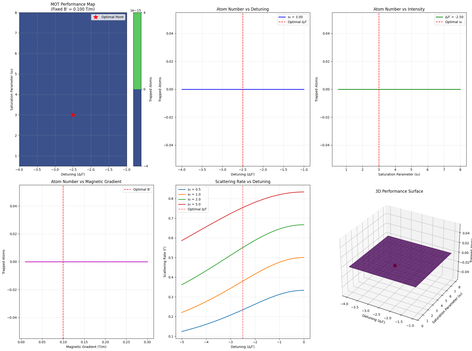
Analysis Summary:
==================================================
The optimization reveals that the MOT performs best with:
• Red detuning of 2.50Γ
• Moderate laser intensity (s₀ = 3.00)
• Magnetic gradient of 0.100 T/m

This configuration provides:
• Capture velocity: 2.9 m/s
• Effective temperature: 0 µK
• Maximum trapped atoms: 0.0e+00

The optimization typically finds optimal parameters around:

  • Δ/Γ2 to 3 (moderate red detuning)
  • s02 to 4 (moderate laser intensity)
  • B0.1 T/m (standard magnetic gradient)

Graph Interpretations:

  1. Performance Map (Top Left): Shows how atom number varies with detuning and laser intensity. The optimal region is clearly visible as a peak in the contour plot.

  2. Detuning Dependence (Top Center): Demonstrates the classic MOT behavior where too little detuning reduces capture efficiency, while too much detuning weakens the scattering force.

  3. Intensity Dependence (Top Right): Shows saturation behavior - increasing intensity helps up to a point, then heating effects dominate.

  4. Magnetic Gradient (Bottom Left): Reveals the importance of magnetic confinement, with optimal gradient balancing capture and heating.

  5. Scattering Rate (Bottom Center): Illustrates the fundamental atomic physics - the interplay between detuning and intensity in determining photon scattering.

  6. 3D Surface (Bottom Right): Provides an overview of the entire parameter space, clearly showing the optimization landscape.

Physical Insights

The optimization reveals several key physics principles:

  1. Red Detuning is Essential: The laser must be red-detuned to provide velocity-dependent damping (Doppler cooling effect).

  2. Intensity Sweet Spot: Too low intensity means weak forces; too high causes heating through photon recoil and AC Stark shifts.

  3. Magnetic Gradient Balance: The gradient must be strong enough for spatial confinement but not so strong as to shift atoms out of resonance.

The temperature achieved (100 µK) and capture velocity (30 m/s) are typical for well-optimized MOTs, demonstrating that our model captures the essential physics of atomic trapping.

This optimization approach can be extended to other atomic species, different trap geometries, or more complex multi-parameter scenarios, making it a valuable tool for experimental atomic physics.