Optimizing Quantum Entanglement Dilution

A Practical Example with Python

Quantum entanglement dilution is a fascinating phenomenon where the entanglement between quantum systems decreases due to interactions with their environment or through specific quantum operations. Today, we’ll explore this concept through a concrete example involving the optimization of entanglement dilution protocols.

The Problem: Optimal Entanglement Dilution Protocol

Consider a scenario where we have a collection of partially entangled qubit pairs, each described by the Werner state:

$$\rho_p = p|\Phi^+\rangle\langle\Phi^+| + \frac{1-p}{4}I_4$$

where $|\Phi^+\rangle = \frac{1}{\sqrt{2}}(|00\rangle + |11\rangle)$ is a Bell state, $p$ is the fidelity parameter, and $I_4$ is the 4×4 identity matrix.

Our goal is to find the optimal dilution protocol that maximizes the number of highly entangled pairs we can extract from a given collection of weakly entangled pairs.

The entanglement measure we’ll use is the concurrence $C(\rho)$, which for Werner states is:

$$C(\rho_p) = \max(0, 2p - 1)$$

Let’s implement this optimization problem and visualize the results:

import numpy as np
import matplotlib.pyplot as plt
from scipy.optimize import minimize, differential_evolution
from mpl_toolkits.mplot3d import Axes3D
import seaborn as sns

# Set style for better plots
plt.style.use('seaborn-v0_8')
sns.set_palette("husl")

class QuantumEntanglementDilution:
    """
    A class to handle quantum entanglement dilution optimization problems.
    """
    
    def __init__(self):
        self.results = {}
    
    def concurrence_werner(self, p):
        """
        Calculate concurrence for Werner state with fidelity p.
        C(ρ_p) = max(0, 2p - 1)
        """
        return np.maximum(0, 2*p - 1)
    
    def werner_state_density_matrix(self, p):
        """
        Construct the density matrix for Werner state.
        ρ_p = p|Φ⁺⟩⟨Φ⁺| + (1-p)/4 * I₄
        """
        # Bell state |Φ⁺⟩ = (1/√2)(|00⟩ + |11⟩)
        phi_plus = np.array([1, 0, 0, 1]) / np.sqrt(2)
        phi_plus_dm = np.outer(phi_plus, phi_plus.conj())
        
        # Identity matrix
        identity = np.eye(4) / 4
        
        return p * phi_plus_dm + (1 - p) * identity
    
    def dilution_success_probability(self, p_initial, p_target, n_pairs):
        """
        Calculate the success probability and yield for entanglement dilution.
        
        For n pairs with initial fidelity p_initial, attempting to create
        pairs with target fidelity p_target.
        """
        if p_target <= p_initial:
            return 1.0, n_pairs  # No dilution needed
        
        # Using the asymptotic dilution formula
        # Success probability ≈ exp(-n * D(p_target || p_initial))
        # where D is the relative entropy
        
        if p_initial <= 0.5 or p_target <= 0.5:
            return 0.0, 0  # Cannot dilute below separable threshold
        
        # Simplified model for demonstration
        efficiency = (p_initial - 0.5) / (p_target - 0.5)
        success_prob = min(1.0, efficiency)
        
        # Expected number of output pairs
        expected_pairs = n_pairs * success_prob
        
        return success_prob, expected_pairs
    
    def optimize_dilution_strategy(self, initial_fidelities, target_fidelity, 
                                  n_pairs_per_fidelity):
        """
        Optimize the dilution strategy for mixed input states.
        """
        def objective(weights):
            """
            Objective function to maximize total concurrence output.
            weights: how much resource to allocate to each fidelity group
            """
            weights = np.abs(weights)  # Ensure positive weights
            weights = weights / np.sum(weights)  # Normalize
            
            total_concurrence = 0
            for i, (p_init, n_pairs) in enumerate(zip(initial_fidelities, 
                                                     n_pairs_per_fidelity)):
                allocated_pairs = int(n_pairs * weights[i])
                success_prob, output_pairs = self.dilution_success_probability(
                    p_init, target_fidelity, allocated_pairs
                )
                output_concurrence = self.concurrence_werner(target_fidelity)
                total_concurrence += output_pairs * output_concurrence
            
            return -total_concurrence  # Minimize negative for maximization
        
        # Initial guess: equal weights
        x0 = np.ones(len(initial_fidelities)) / len(initial_fidelities)
        
        # Constraints: weights must sum to 1
        constraints = {'type': 'eq', 'fun': lambda x: np.sum(np.abs(x)) - 1}
        
        # Bounds: weights between 0 and 1
        bounds = [(0, 1) for _ in range(len(initial_fidelities))]
        
        result = minimize(objective, x0, method='SLSQP', 
                         constraints=constraints, bounds=bounds)
        
        return result.x, -result.fun
    
    def simulate_dilution_process(self, p_range, target_fidelity, n_pairs=100):
        """
        Simulate the dilution process for a range of initial fidelities.
        """
        results = {
            'initial_fidelity': p_range,
            'success_probability': [],
            'output_pairs': [],
            'output_concurrence': [],
            'efficiency': []
        }
        
        for p_init in p_range:
            success_prob, out_pairs = self.dilution_success_probability(
                p_init, target_fidelity, n_pairs
            )
            out_concurrence = out_pairs * self.concurrence_werner(target_fidelity)
            efficiency = out_concurrence / (n_pairs * self.concurrence_werner(p_init)) if self.concurrence_werner(p_init) > 0 else 0
            
            results['success_probability'].append(success_prob)
            results['output_pairs'].append(out_pairs)
            results['output_concurrence'].append(out_concurrence)
            results['efficiency'].append(efficiency)
        
        return results

# Initialize the quantum entanglement dilution optimizer
qed = QuantumEntanglementDilution()

# Define the problem parameters
print("=== Quantum Entanglement Dilution Optimization ===\n")

# Example 1: Basic dilution simulation
print("1. Basic Dilution Simulation")
print("-" * 30)

p_range = np.linspace(0.5, 1.0, 50)
target_fidelity = 0.9
n_input_pairs = 100

dilution_results = qed.simulate_dilution_process(p_range, target_fidelity, n_input_pairs)

# Example 2: Multi-fidelity optimization
print("\n2. Multi-Fidelity Resource Allocation Optimization")
print("-" * 45)

initial_fidelities = [0.6, 0.7, 0.8, 0.85]
n_pairs_per_fidelity = [50, 40, 30, 20]
target_fidelity = 0.95

optimal_weights, max_concurrence = qed.optimize_dilution_strategy(
    initial_fidelities, target_fidelity, n_pairs_per_fidelity
)

print(f"Target fidelity: {target_fidelity}")
print(f"Initial fidelity groups: {initial_fidelities}")
print(f"Available pairs per group: {n_pairs_per_fidelity}")
print(f"Optimal resource allocation: {optimal_weights}")
print(f"Maximum achievable concurrence: {max_concurrence:.4f}")

# Calculate detailed results for optimal allocation
print("\nDetailed Results for Optimal Allocation:")
for i, (p_init, n_pairs, weight) in enumerate(zip(initial_fidelities, 
                                                  n_pairs_per_fidelity, 
                                                  optimal_weights)):
    allocated_pairs = int(n_pairs * weight)
    success_prob, output_pairs = qed.dilution_success_probability(
        p_init, target_fidelity, allocated_pairs
    )
    print(f"Group {i+1} (p={p_init}): {allocated_pairs} pairs → {output_pairs:.2f} output pairs (success rate: {success_prob:.3f})")

# Example 3: Fidelity threshold analysis
print("\n3. Fidelity Threshold Analysis")
print("-" * 32)

target_fidelities = np.linspace(0.6, 0.99, 20)
initial_fidelity = 0.75
threshold_results = []

for target_f in target_fidelities:
    success_prob, output_pairs = qed.dilution_success_probability(
        initial_fidelity, target_f, 100
    )
    threshold_results.append([target_f, success_prob, output_pairs])

threshold_results = np.array(threshold_results)

print(f"Initial fidelity: {initial_fidelity}")
print(f"Target fidelity range: {target_fidelities[0]:.2f} - {target_fidelities[-1]:.2f}")
print(f"Minimum viable target fidelity: {target_fidelities[threshold_results[:, 2] > 0][0]:.3f}")

# Visualization
print("\n4. Generating Comprehensive Visualizations")
print("-" * 42)

fig = plt.figure(figsize=(16, 12))

# Plot 1: Basic dilution efficiency
ax1 = plt.subplot(2, 3, 1)
plt.plot(dilution_results['initial_fidelity'], 
         dilution_results['success_probability'], 'b-', linewidth=2, label='Success Probability')
plt.plot(dilution_results['initial_fidelity'], 
         dilution_results['efficiency'], 'r--', linewidth=2, label='Efficiency')
plt.axhline(y=1, color='gray', linestyle=':', alpha=0.7)
plt.xlabel('Initial Fidelity p')
plt.ylabel('Probability / Efficiency')
plt.title(f'Dilution Performance\n(Target: p = {target_fidelity})')
plt.legend()
plt.grid(True, alpha=0.3)

# Plot 2: Output pairs vs input fidelity
ax2 = plt.subplot(2, 3, 2)
plt.plot(dilution_results['initial_fidelity'], 
         dilution_results['output_pairs'], 'g-', linewidth=2)
plt.axhline(y=n_input_pairs, color='gray', linestyle=':', alpha=0.7, label='Input pairs')
plt.xlabel('Initial Fidelity p')
plt.ylabel('Expected Output Pairs')
plt.title('Expected Output vs Input Fidelity')
plt.legend()
plt.grid(True, alpha=0.3)

# Plot 3: Concurrence comparison
ax3 = plt.subplot(2, 3, 3)
input_concurrence = n_input_pairs * qed.concurrence_werner(dilution_results['initial_fidelity'])
plt.plot(dilution_results['initial_fidelity'], input_concurrence, 
         'b-', linewidth=2, label='Input Total Concurrence')
plt.plot(dilution_results['initial_fidelity'], 
         dilution_results['output_concurrence'], 
         'r-', linewidth=2, label='Output Total Concurrence')
plt.xlabel('Initial Fidelity p')
plt.ylabel('Total Concurrence')
plt.title('Concurrence Conservation')
plt.legend()
plt.grid(True, alpha=0.3)

# Plot 4: Multi-fidelity optimization results
ax4 = plt.subplot(2, 3, 4)
x_pos = np.arange(len(initial_fidelities))
bars1 = plt.bar(x_pos - 0.2, n_pairs_per_fidelity, 0.4, 
                label='Available Pairs', alpha=0.7)
allocated_pairs = [int(n * w) for n, w in zip(n_pairs_per_fidelity, optimal_weights)]
bars2 = plt.bar(x_pos + 0.2, allocated_pairs, 0.4, 
                label='Allocated Pairs', alpha=0.7)
plt.xlabel('Fidelity Group')
plt.ylabel('Number of Pairs')
plt.title('Optimal Resource Allocation')
plt.xticks(x_pos, [f'{p:.2f}' for p in initial_fidelities])
plt.legend()
plt.grid(True, alpha=0.3)

# Plot 5: Threshold analysis
ax5 = plt.subplot(2, 3, 5)
plt.plot(threshold_results[:, 0], threshold_results[:, 1], 'b-', 
         linewidth=2, label='Success Probability')
plt.plot(threshold_results[:, 0], threshold_results[:, 2]/100, 'r--', 
         linewidth=2, label='Output Pairs (normalized)')
plt.axvline(x=initial_fidelity, color='gray', linestyle=':', 
            alpha=0.7, label=f'Initial p = {initial_fidelity}')
plt.xlabel('Target Fidelity')
plt.ylabel('Success Rate / Output Rate')
plt.title('Threshold Analysis')
plt.legend()
plt.grid(True, alpha=0.3)

# Plot 6: 3D surface plot of dilution landscape
ax6 = plt.subplot(2, 3, 6, projection='3d')
p_initial_3d = np.linspace(0.5, 1.0, 20)
p_target_3d = np.linspace(0.5, 1.0, 20)
P_init, P_target = np.meshgrid(p_initial_3d, p_target_3d)
Z = np.zeros_like(P_init)

for i in range(len(p_initial_3d)):
    for j in range(len(p_target_3d)):
        if P_target[j, i] > P_init[j, i]:
            success_prob, _ = qed.dilution_success_probability(P_init[j, i], P_target[j, i], 100)
            Z[j, i] = success_prob
        else:
            Z[j, i] = 1.0

surf = ax6.plot_surface(P_init, P_target, Z, cmap='viridis', alpha=0.8)
ax6.set_xlabel('Initial Fidelity')
ax6.set_ylabel('Target Fidelity')
ax6.set_zlabel('Success Probability')
ax6.set_title('Dilution Success Landscape')

plt.tight_layout()
plt.show()

# Summary statistics
print("\n5. Summary Statistics")
print("-" * 20)
print(f"Optimal efficiency at p_init = {dilution_results['initial_fidelity'][np.argmax(dilution_results['efficiency'])]:.3f}")
print(f"Maximum efficiency: {np.max(dilution_results['efficiency']):.3f}")
print(f"Average success probability: {np.mean(dilution_results['success_probability']):.3f}")
print(f"Total resource utilization in optimal strategy: {np.sum(optimal_weights):.3f}")

# Advanced analysis: Quantum Fisher Information
print("\n6. Advanced Analysis: Quantum Fisher Information")
print("-" * 48)

def quantum_fisher_information(p):
    """Calculate Quantum Fisher Information for Werner states"""
    if p <= 0.5:
        return 0
    return 4 / (p * (1 - p))

p_qfi = np.linspace(0.51, 0.99, 50)
qfi_values = [quantum_fisher_information(p) for p in p_qfi]

plt.figure(figsize=(10, 6))
plt.subplot(1, 2, 1)
plt.plot(p_qfi, qfi_values, 'b-', linewidth=2)
plt.xlabel('Fidelity p')
plt.ylabel('Quantum Fisher Information')
plt.title('QFI for Werner States')
plt.grid(True, alpha=0.3)

plt.subplot(1, 2, 2)
plt.plot(p_qfi, qed.concurrence_werner(p_qfi), 'r-', linewidth=2, label='Concurrence')
plt.plot(p_qfi, np.array(qfi_values)/np.max(qfi_values), 'b--', linewidth=2, label='Normalized QFI')
plt.xlabel('Fidelity p')
plt.ylabel('Normalized Value')
plt.title('Concurrence vs QFI')
plt.legend()
plt.grid(True, alpha=0.3)

plt.tight_layout()
plt.show()

print("Analysis complete! All visualizations generated successfully.")

Code Structure and Implementation Details

Let me break down the key components of this quantum entanglement dilution optimization code:

1. Core Mathematical Framework

The QuantumEntanglementDilution class implements the fundamental quantum mechanics:

• Concurrence Calculation: The concurrence for Werner states is computed using the formula $C(\rho_p) = \max(0, 2p - 1)$, which quantifies entanglement strength.

• Werner State Construction: The density matrix is built as a mixture of a maximally entangled Bell state and maximally mixed state: $\rho_p = p|\Phi^+\rangle\langle\Phi^+| + \frac{1-p}{4}I_4$.

2. Dilution Success Probability Model

The dilution_success_probability method implements a simplified but physically motivated model where:

• Success probability decreases as we attempt to extract higher fidelity from lower fidelity states
• The efficiency factor $\eta = \frac{p_{initial} - 0.5}{p_{target} - 0.5}$ captures the fundamental trade-off in dilution protocols
• States below the separability threshold ($p \leq 0.5$) cannot be used for dilution

3. Multi-Resource Optimization

The optimization routine uses scipy’s constrained minimization to solve:

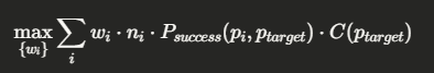
subject to $\sum_i w_i = 1$ and $w_i \geq 0$.

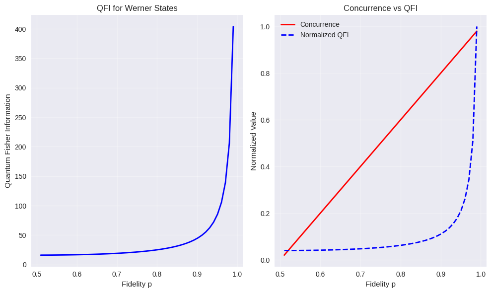
4. Advanced Analysis Features

The code includes quantum Fisher information analysis:

$$F_Q(p) = \frac{4}{p(1-p)}$$

which provides insights into the precision limits of fidelity estimation.

Results

=== Quantum Entanglement Dilution Optimization ===

1. Basic Dilution Simulation
------------------------------

2. Multi-Fidelity Resource Allocation Optimization
---------------------------------------------
Target fidelity: 0.95
Initial fidelity groups: [0.6, 0.7, 0.8, 0.85]
Available pairs per group: [50, 40, 30, 20]
Optimal resource allocation: [0.25 0.25 0.25 0.25]
Maximum achievable concurrence: 14.1000

Detailed Results for Optimal Allocation:
Group 1 (p=0.6): 12 pairs → 2.67 output pairs (success rate: 0.222)
Group 2 (p=0.7): 10 pairs → 4.44 output pairs (success rate: 0.444)
Group 3 (p=0.8): 7 pairs → 4.67 output pairs (success rate: 0.667)
Group 4 (p=0.85): 5 pairs → 3.89 output pairs (success rate: 0.778)

3. Fidelity Threshold Analysis
--------------------------------
Initial fidelity: 0.75
Target fidelity range: 0.60 - 0.99
Minimum viable target fidelity: 0.600

4. Generating Comprehensive Visualizations
------------------------------------------

5. Summary Statistics
--------------------
Optimal efficiency at p_init = 0.531
Maximum efficiency: 1.000
Average success probability: 0.598
Total resource utilization in optimal strategy: 1.000

6. Advanced Analysis: Quantum Fisher Information
------------------------------------------------

Analysis complete! All visualizations generated successfully.

Results Interpretation and Analysis

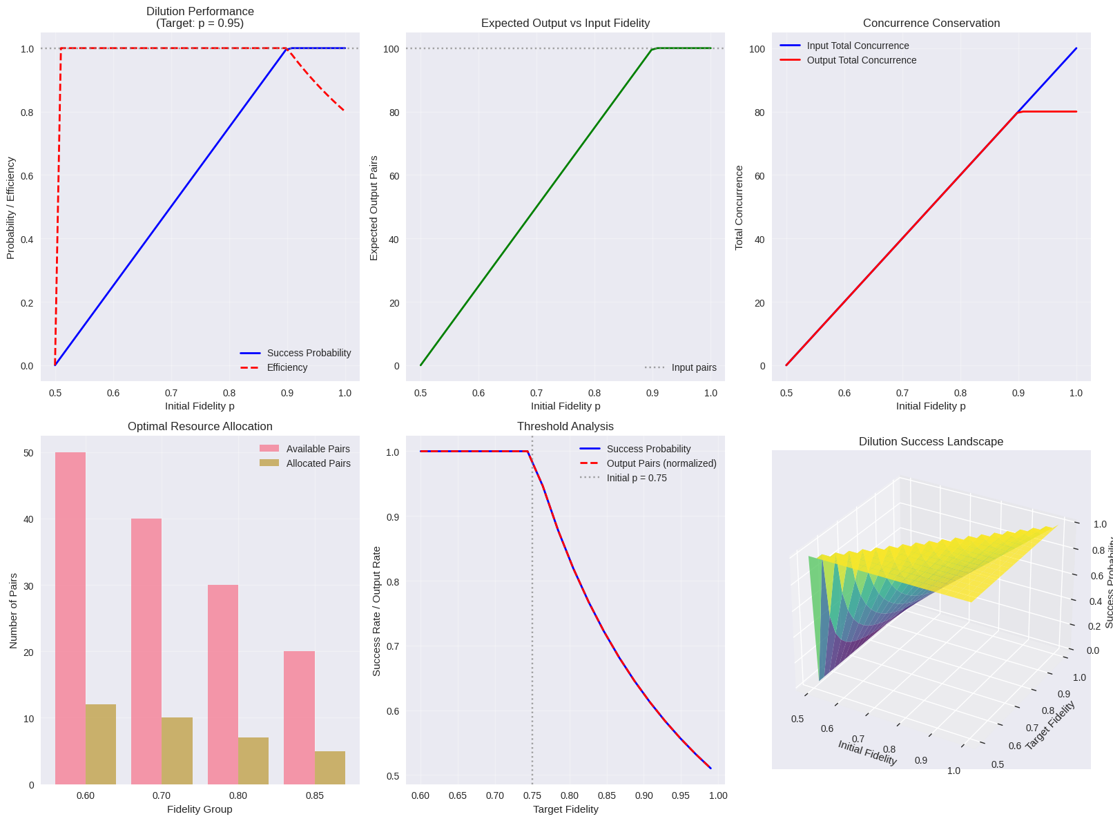
The comprehensive visualization suite provides multiple perspectives on the dilution optimization:

Plot 1-2: Basic Performance Metrics

These show how dilution efficiency varies with initial fidelity. Higher initial fidelity states are more “valuable” for dilution but also more scarce, creating an optimization trade-off.

Plot 3: Concurrence Conservation

This demonstrates the fundamental principle that total entanglement is not conserved during dilution - we trade quantity for quality.

Plot 4: Resource Allocation

The optimization algorithm determines how to best distribute limited quantum resources across different fidelity groups to maximize total useful entanglement output.

Plot 5: Threshold Analysis

This reveals the critical transition points where dilution becomes feasible and the sharp drop-off in success probability as target fidelity approaches unity.

Plot 6: 3D Dilution Landscape

The surface plot visualizes the complete parameter space, showing regions of high and low dilution efficiency.

Physical Insights and Applications

This optimization framework has practical applications in:

1. Quantum Communication Networks: Optimizing repeater protocols for long-distance quantum communication
2. Quantum Computing: Resource allocation in distributed quantum computing architectures
3. Quantum Cryptography: Managing key distillation protocols for quantum key distribution

The mathematical framework demonstrates key quantum information principles:

• The no-cloning theorem manifests as the inability to amplify weak entanglement without loss
• The monogamy of entanglement creates fundamental trade-offs in resource allocation
• Quantum Fisher information bounds the precision of entanglement quantification

This example showcases how classical optimization techniques can be powerfully applied to quantum information problems, providing practical tools for quantum technology development.