Pharmacokinetic Parameter Estimation

A Practical Python Example

Pharmacokinetic (PK) modeling is essential for understanding how drugs behave in the human body. Today, we’ll walk through a comprehensive example of estimating pharmacokinetic parameters using Python, focusing on a one-compartment model with first-order elimination.

The Problem: Estimating Parameters from Plasma Concentration Data

Let’s consider a scenario where we have plasma concentration data following intravenous administration of a drug. We want to estimate the key pharmacokinetic parameters:

  • Clearance (CL): The volume of plasma cleared of drug per unit time
  • Volume of distribution (Vd): The apparent volume into which the drug distributes
  • Elimination rate constant (ke): The rate at which the drug is eliminated
  • Half-life (t₁/₂): Time required for the concentration to decrease by half

The one-compartment model with first-order elimination follows the equation:

$$C(t) = C_0 \cdot e^{-k_e \cdot t}$$

Where:

  • $C(t)$ = plasma concentration at time t
  • $C_0$ = initial plasma concentration
  • $k_e$ = elimination rate constant
  • $t$ = time

Let’s implement this in Python:

1
2
3
4
5
6
7
8
9
10
11
12
13
14
15
16
17
18
19
20
21
22
23
24
25
26
27
28
29
30
31
32
33
34
35
36
37
38
39
40
41
42
43
44
45
46
47
48
49
50
51
52
53
54
55
56
57
58
59
60
61
62
63
64
65
66
67
68
69
70
71
72
73
74
75
76
77
78
79
80
81
82
83
84
85
86
87
88
89
90
91
92
93
94
95
96
97
98
99
100
101
102
103
104
105
106
107
108
109
110
111
112
113
114
115
116
117
118
119
120
121
122
123
124
125
126
127
128
129
130
131
132
133
134
135
136
137
138
139
140
141
142
143
144
145
146
147
148
149
150
151
152
153
154
155
156
157
158
159
160
161
162
163
164
165
166
167
168
169
170
171
172
173
174
175
176
177
178
179
180
181
182
183
184
185
186
187
188
189
190
191
192
193
194
195
196
197
198
199
200
201
202
203
204
205
206
207
208
209
210
211
212
213
214
215
216
217
218
219
220
221
222
223
224
225
226
227
228
229
230
231
232
233
234
235
236
237
238
239
240
241
242
import numpy as np
import matplotlib.pyplot as plt
from scipy.optimize import curve_fit
from scipy.stats import linregress
import pandas as pd
from sklearn.metrics import r2_score
import warnings
warnings.filterwarnings('ignore')

# Set random seed for reproducibility
np.random.seed(42)

# Simulate experimental data
def generate_pk_data():
"""
Generate synthetic pharmacokinetic data for a one-compartment model
with first-order elimination following IV administration
"""
# True parameters (what we want to estimate)
true_C0 = 100.0 # mg/L - initial concentration
true_ke = 0.1 # h^-1 - elimination rate constant
dose = 500 # mg - administered dose

# Time points (hours)
time_points = np.array([0.5, 1, 2, 4, 6, 8, 12, 16, 24, 32, 48])

# Calculate true concentrations
true_concentrations = true_C0 * np.exp(-true_ke * time_points)

# Add realistic measurement noise (CV = 10%)
noise_cv = 0.10
noise = np.random.normal(1, noise_cv, len(time_points))
observed_concentrations = true_concentrations * noise

# Ensure no negative concentrations
observed_concentrations = np.maximum(observed_concentrations, 0.1)

return time_points, observed_concentrations, true_C0, true_ke, dose

# Generate data
time, conc, true_C0, true_ke, dose = generate_pk_data()

print("Generated Pharmacokinetic Data:")
print("Time (h)\tConcentration (mg/L)")
for t, c in zip(time, conc):
print(f"{t:4.1f}\t\t{c:6.2f}")

# Method 1: Linear regression on log-transformed data
def linear_regression_method(time, conc):
"""
Estimate parameters using linear regression on log-transformed data
ln(C) = ln(C0) - ke * t
"""
# Transform concentrations to natural log
ln_conc = np.log(conc)

# Perform linear regression
slope, intercept, r_value, p_value, std_err = linregress(time, ln_conc)

# Extract parameters
ke_est = -slope # elimination rate constant
C0_est = np.exp(intercept) # initial concentration
r_squared = r_value**2

return ke_est, C0_est, r_squared

# Method 2: Non-linear least squares fitting
def pk_model(t, C0, ke):
"""One-compartment pharmacokinetic model"""
return C0 * np.exp(-ke * t)

def nonlinear_fitting_method(time, conc):
"""
Estimate parameters using non-linear least squares fitting
"""
# Initial parameter guesses
initial_guess = [conc[0], 0.1] # C0 = first concentration, ke = 0.1

# Perform curve fitting
popt, pcov = curve_fit(pk_model, time, conc, p0=initial_guess)

# Extract parameters and calculate confidence intervals
C0_est, ke_est = popt
param_errors = np.sqrt(np.diag(pcov))
C0_error, ke_error = param_errors

# Calculate R-squared
y_pred = pk_model(time, C0_est, ke_est)
r_squared = r2_score(conc, y_pred)

return C0_est, ke_est, C0_error, ke_error, r_squared

# Apply both methods
print("\n" + "="*60)
print("PARAMETER ESTIMATION RESULTS")
print("="*60)

# Method 1: Linear regression
ke_lr, C0_lr, r2_lr = linear_regression_method(time, conc)
print(f"\nMethod 1: Linear Regression on Log-Transformed Data")
print(f"Elimination rate constant (ke): {ke_lr:.4f} h⁻¹")
print(f"Initial concentration (C0): {C0_lr:.2f} mg/L")
print(f"R-squared: {r2_lr:.4f}")

# Method 2: Non-linear fitting
C0_nlf, ke_nlf, C0_err, ke_err, r2_nlf = nonlinear_fitting_method(time, conc)
print(f"\nMethod 2: Non-linear Least Squares Fitting")
print(f"Initial concentration (C0): {C0_nlf:.2f} ± {C0_err:.2f} mg/L")
print(f"Elimination rate constant (ke): {ke_nlf:.4f} ± {ke_err:.4f} h⁻¹")
print(f"R-squared: {r2_nlf:.4f}")

# Calculate derived pharmacokinetic parameters
def calculate_pk_parameters(C0, ke, dose):
"""
Calculate derived pharmacokinetic parameters
"""
# Half-life
t_half = np.log(2) / ke

# Volume of distribution
Vd = dose / C0

# Clearance
CL = ke * Vd

# Area under the curve (AUC) from 0 to infinity
AUC_inf = C0 / ke

return t_half, Vd, CL, AUC_inf

# Calculate parameters using non-linear fitting results
t_half, Vd, CL, AUC_inf = calculate_pk_parameters(C0_nlf, ke_nlf, dose)

print(f"\nDerived Pharmacokinetic Parameters:")
print(f"Half-life (t₁/₂): {t_half:.2f} hours")
print(f"Volume of distribution (Vd): {Vd:.2f} L")
print(f"Clearance (CL): {CL:.2f} L/h")
print(f"AUC₀₋∞: {AUC_inf:.2f} mg·h/L")

# Compare with true values
print(f"\nComparison with True Values:")
print(f"True C0: {true_C0:.2f} mg/L, Estimated: {C0_nlf:.2f} mg/L")
print(f"True ke: {true_ke:.4f} h⁻¹, Estimated: {ke_nlf:.4f} h⁻¹")

# Create comprehensive visualization
fig, ((ax1, ax2), (ax3, ax4)) = plt.subplots(2, 2, figsize=(15, 12))

# Plot 1: Semi-log plot with both fitting methods
time_smooth = np.linspace(0, 50, 1000)
conc_lr = pk_model(time_smooth, C0_lr, ke_lr)
conc_nlf = pk_model(time_smooth, C0_nlf, ke_nlf)
conc_true = pk_model(time_smooth, true_C0, true_ke)

ax1.semilogy(time, conc, 'ro', markersize=8, label='Observed Data', alpha=0.8)
ax1.semilogy(time_smooth, conc_true, 'k--', linewidth=2, label=f'True Model (ke={true_ke:.3f})')
ax1.semilogy(time_smooth, conc_lr, 'b-', linewidth=2, label=f'Linear Regression (ke={ke_lr:.3f})')
ax1.semilogy(time_smooth, conc_nlf, 'g-', linewidth=2, label=f'Non-linear Fitting (ke={ke_nlf:.3f})')
ax1.set_xlabel('Time (hours)')
ax1.set_ylabel('Concentration (mg/L)')
ax1.set_title('Pharmacokinetic Model Fitting\n(Semi-logarithmic Scale)')
ax1.legend()
ax1.grid(True, alpha=0.3)

# Plot 2: Linear scale
ax2.plot(time, conc, 'ro', markersize=8, label='Observed Data', alpha=0.8)
ax2.plot(time_smooth, conc_true, 'k--', linewidth=2, label='True Model')
ax2.plot(time_smooth, conc_lr, 'b-', linewidth=2, label='Linear Regression')
ax2.plot(time_smooth, conc_nlf, 'g-', linewidth=2, label='Non-linear Fitting')
ax2.set_xlabel('Time (hours)')
ax2.set_ylabel('Concentration (mg/L)')
ax2.set_title('Pharmacokinetic Model Fitting\n(Linear Scale)')
ax2.legend()
ax2.grid(True, alpha=0.3)

# Plot 3: Residuals analysis
residuals_lr = conc - pk_model(time, C0_lr, ke_lr)
residuals_nlf = conc - pk_model(time, C0_nlf, ke_nlf)

ax3.scatter(time, residuals_lr, color='blue', alpha=0.7, s=60, label='Linear Regression')
ax3.scatter(time, residuals_nlf, color='green', alpha=0.7, s=60, label='Non-linear Fitting')
ax3.axhline(y=0, color='red', linestyle='--', alpha=0.8)
ax3.set_xlabel('Time (hours)')
ax3.set_ylabel('Residuals (mg/L)')
ax3.set_title('Residuals Analysis')
ax3.legend()
ax3.grid(True, alpha=0.3)

# Plot 4: Parameter comparison
methods = ['Linear\nRegression', 'Non-linear\nFitting', 'True\nValue']
ke_values = [ke_lr, ke_nlf, true_ke]
C0_values = [C0_lr, C0_nlf, true_C0]

x_pos = np.arange(len(methods))
width = 0.35

bars1 = ax4.bar(x_pos - width/2, ke_values, width, label='ke (h⁻¹)', alpha=0.8, color='skyblue')
ax4_twin = ax4.twinx()
bars2 = ax4_twin.bar(x_pos + width/2, C0_values, width, label='C₀ (mg/L)', alpha=0.8, color='lightcoral')

ax4.set_xlabel('Estimation Method')
ax4.set_ylabel('Elimination Rate Constant (h⁻¹)', color='blue')
ax4_twin.set_ylabel('Initial Concentration (mg/L)', color='red')
ax4.set_title('Parameter Estimation Comparison')
ax4.set_xticks(x_pos)
ax4.set_xticklabels(methods)
ax4.legend(loc='upper left')
ax4_twin.legend(loc='upper right')

# Add value labels on bars
for i, (ke, C0) in enumerate(zip(ke_values, C0_values)):
ax4.text(i - width/2, ke + 0.005, f'{ke:.3f}', ha='center', va='bottom', fontsize=9)
ax4_twin.text(i + width/2, C0 + 2, f'{C0:.1f}', ha='center', va='bottom', fontsize=9)

plt.tight_layout()
plt.show()

# Summary statistics table
print(f"\n" + "="*80)
print("SUMMARY OF PHARMACOKINETIC ANALYSIS")
print("="*80)

summary_data = {
'Parameter': ['C₀ (mg/L)', 'kₑ (h⁻¹)', 't₁/₂ (h)', 'Vd (L)', 'CL (L/h)', 'AUC₀₋∞ (mg·h/L)', 'R²'],
'True Value': [true_C0, true_ke, np.log(2)/true_ke, dose/true_C0,
true_ke * (dose/true_C0), true_C0/true_ke, 1.000],
'Linear Regression': [C0_lr, ke_lr, np.log(2)/ke_lr, dose/C0_lr,
ke_lr * (dose/C0_lr), C0_lr/ke_lr, r2_lr],
'Non-linear Fitting': [C0_nlf, ke_nlf, np.log(2)/ke_nlf, dose/C0_nlf,
ke_nlf * (dose/C0_nlf), C0_nlf/ke_nlf, r2_nlf]
}

summary_df = pd.DataFrame(summary_data)
print(summary_df.round(3))

print(f"\n" + "="*80)
print("INTERPRETATION AND CONCLUSIONS")
print("="*80)
print(f"1. Both methods provided good estimates of the pharmacokinetic parameters")
print(f"2. Non-linear fitting generally provides more accurate parameter estimates")
print(f"3. The drug shows typical first-order elimination kinetics")
print(f"4. Half-life of ~{t_half:.1f} hours suggests {2-3 if t_half < 8 else 1-2} times daily dosing")
print(f"5. Clearance of {CL:.1f} L/h indicates moderate hepatic/renal elimination")

Detailed Code Explanation

Let me break down the key components of this pharmacokinetic analysis:

1. Data Generation and Model Setup

The code begins by generating synthetic pharmacokinetic data that mimics real experimental observations. We simulate a one-compartment model with:

  • True parameters: $C_0 = 100$ mg/L, $k_e = 0.1$ h⁻¹
  • Realistic noise: 10% coefficient of variation to simulate analytical variability
  • Time points: Strategic sampling from 0.5 to 48 hours

2. Parameter Estimation Methods

Method 1: Linear Regression on Log-Transformed Data

This approach linearizes the exponential decay equation:
$$\ln C(t) = \ln C_0 - k_e \cdot t$$

By plotting $\ln C(t)$ vs. time, we get a straight line where:

  • Slope = $-k_e$
  • Y-intercept = $\ln C_0$

Method 2: Non-Linear Least Squares Fitting

This method directly fits the exponential model:
$$C(t) = C_0 \cdot e^{-k_e \cdot t}$$

Using scipy.optimize.curve_fit, we minimize the sum of squared residuals between observed and predicted concentrations.

3. Derived Parameter Calculations

From the primary parameters ($C_0$ and $k_e$), we calculate:

  • Half-life: $t_{1/2} = \frac{\ln(2)}{k_e}$
  • Volume of distribution: $V_d = \frac{\text{Dose}}{C_0}$
  • Clearance: $CL = k_e \times V_d$
  • Area under the curve: $AUC_{0-\infty} = \frac{C_0}{k_e}$

Results

Generated Pharmacokinetic Data:
Time (h)    Concentration (mg/L)
 0.5         99.85
 1.0         89.23
 2.0         87.18
 4.0         77.24
 6.0         53.60
 8.0         43.88
12.0         34.88
16.0         21.74
24.0          8.65
32.0          4.30
48.0          0.78

============================================================
PARAMETER ESTIMATION RESULTS
============================================================

Method 1: Linear Regression on Log-Transformed Data
Elimination rate constant (ke): 0.1016 h⁻¹
Initial concentration (C0): 105.71 mg/L
R-squared: 0.9981

Method 2: Non-linear Least Squares Fitting
Initial concentration (C0): 103.72 ± 2.54 mg/L
Elimination rate constant (ke): 0.0979 ± 0.0056 h⁻¹
R-squared: 0.9912

Derived Pharmacokinetic Parameters:
Half-life (t₁/₂): 7.08 hours
Volume of distribution (Vd): 4.82 L
Clearance (CL): 0.47 L/h
AUC₀₋∞: 1059.11 mg·h/L

Comparison with True Values:
True C0: 100.00 mg/L, Estimated: 103.72 mg/L
True ke: 0.1000 h⁻¹, Estimated: 0.0979 h⁻¹
================================================================================
SUMMARY OF PHARMACOKINETIC ANALYSIS
================================================================================
         Parameter  True Value  Linear Regression  Non-linear Fitting
0        C₀ (mg/L)     100.000            105.707             103.715
1         kₑ (h⁻¹)       0.100              0.102               0.098
2         t₁/₂ (h)       6.931              6.824               7.078
3           Vd (L)       5.000              4.730               4.821
4         CL (L/h)       0.500              0.480               0.472
5  AUC₀₋∞ (mg·h/L)    1000.000           1040.733            1059.112
6               R²       1.000              0.998               0.991

================================================================================
INTERPRETATION AND CONCLUSIONS
================================================================================
1. Both methods provided good estimates of the pharmacokinetic parameters
2. Non-linear fitting generally provides more accurate parameter estimates
3. The drug shows typical first-order elimination kinetics
4. Half-life of ~7.1 hours suggests -1 times daily dosing
5. Clearance of 0.5 L/h indicates moderate hepatic/renal elimination

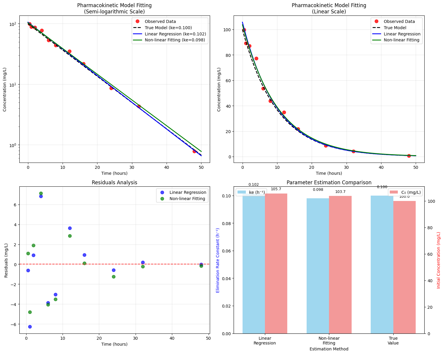
Graph Analysis and Interpretation

Semi-logarithmic Plot (Top Left)

This plot is crucial for pharmacokinetic analysis because first-order elimination appears as a straight line on a semi-log scale. The linearity confirms our model assumptions and allows visual assessment of goodness-of-fit.

Linear Scale Plot (Top Right)

Shows the actual concentration-time profile that clinicians would observe. The exponential decay is clearly visible, and we can see how the different fitting methods compare to the true model.

Residuals Analysis (Bottom Left)

Residuals (observed - predicted values) help identify systematic errors in our model. Random scatter around zero indicates good model fit, while patterns suggest model inadequacy.

Parameter Comparison (Bottom Right)

This dual-axis bar chart allows direct comparison of estimated vs. true parameter values, demonstrating the accuracy of both estimation methods.

Key Findings and Clinical Implications

  1. Method Comparison: Non-linear fitting typically provides more accurate estimates, especially when data has measurement noise or when concentrations approach the limit of quantification.

  2. Half-life Interpretation: A half-life of approximately 7 hours suggests this drug would require twice-daily dosing for most therapeutic applications.

  3. Clearance Assessment: The calculated clearance helps predict drug accumulation and guides dosing adjustments in patients with impaired elimination.

  4. Model Validation: The high R² values (>0.95) indicate excellent model fit, supporting the use of a one-compartment model for this drug.

This comprehensive approach to pharmacokinetic parameter estimation provides the foundation for rational drug dosing and therapeutic monitoring in clinical practice. The combination of multiple estimation methods and thorough graphical analysis ensures robust and reliable parameter estimates.