🔧 A Python Walkthrough
In this post, we’ll dive into the classic scheduling problem: how do we assign a set of jobs to a limited number of machines so that the total processing time—also known as the makespan—is minimized?
We’ll model a simple but powerful version of this problem and solve it using Python
Along the way, we’ll visualize the results for better understanding.
🧩 Problem Overview
Imagine we have n jobs and m machines.
Each job takes a certain amount of time to complete, and our goal is to assign jobs to machines such that:
- Each job is assigned to exactly one machine
- The total completion time (makespan) is minimized
This is known as the Minimum Makespan Scheduling Problem, and can be formally expressed as:
$$
\text{Minimize } \max_{i \in {1, \dots, m}} \sum_{j \in J_i} p_j
$$
Where:
- $p_j$ is the processing time of job $j$
- $J_i$ is the set of jobs assigned to machine $i$
We’ll solve this with a greedy heuristic known as the Longest Processing Time first (LPT) rule.
⚙️ Sample Scenario
Let’s say we have:
- 10 jobs with varying processing times
- 3 machines
Let’s implement and solve it!
💻 Python Code
1 | import matplotlib.pyplot as plt |
🔍 Code Explanation
1. Input Definition
We define:
num_machines: how many machines we havenum_jobs: how many jobs need to be scheduledjobs: randomly generated list of processing times
1 | jobs = [random.randint(2, 20) for _ in range(num_jobs)] |
2. LPT Sorting
The LPT heuristic tells us to assign longest jobs first, so we sort the jobs in descending order.
1 | jobs_sorted = sorted(enumerate(jobs), key=lambda x: -x[1]) |
3. Greedy Assignment
Each job is assigned to the machine with the current minimum load.
1 | min_machine = machine_loads.index(min(machine_loads)) |
This ensures we balance the load as efficiently as possible at each step.
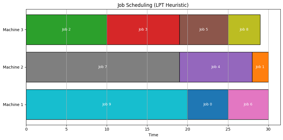
4. Gantt Chart Visualization
To visualize the job distribution over time across machines, we use a horizontal bar chart where each bar represents a job.
- Bars are placed sequentially on the time axis.
- The chart clearly shows the job sequence and load on each machine.
📈 Results & Analysis
Each machine’s workload is printed and visualized.
For example, the output might look like:
1 | Machine 1: [(9, 20), (0, 5), (6, 5)] (Total: 30) |
From this, you can see:
- Machines 3 have a lower total load
- Machine 1 and 2 ended up with the highest load (i.e., the makespan)
Thus, the makespan is:
$$
\text{Makespan} = \max([30, 30, 29]) = 30
$$
The visualization helps you instantly grasp the load imbalance.
🧠 Conclusion
While the LPT heuristic doesn’t guarantee an optimal solution, it’s fast and effective, and often yields a near-optimal result.
✅ Pros:
- Easy to implement
- Fast even for large job sets
⚠️ Cons:
- Not always optimal
- Doesn’t handle job dependencies or setup times
For larger or more complex scheduling problems, consider advanced methods like:
- Integer Linear Programming (ILP)
- Constraint Programming
- Metaheuristics (e.g., Genetic Algorithms)