📊 A Data-Driven Python Approach
In today’s fast-paced e-commerce and retail environment, finding the optimal price that balances demand and revenue is a cornerstone of profitability.
But this is no longer a guessing game.
Thanks to machine learning and optimization, we can forecast demand based on historical data and optimize pricing accordingly.
In this post, we’ll walk through a concrete example of this integration using Python, forecasting demand with linear regression and then using that to maximize revenue through optimization.
🔍 Problem Overview
We have historical data containing:
- Prices at which a product was sold
- Corresponding units sold
We want to:
- Forecast demand based on price using linear regression.
- Optimize price to maximize expected revenue.
The Revenue Function
Let:
- $p$ be the price
- $D(p)$ be the demand at price $p$
Then:
$$
\text{Revenue}(p) = p \cdot D(p)
$$
We’ll forecast $D(p)$ with a simple linear regression:
$$
D(p) = a - b \cdot p
$$
Where $a, b$ are learned from data.
📁 Step 1: Python Code – Forecasting + Optimization
Let’s start with the full code, then break it down step-by-step.
1 | import numpy as np |
🧠 Code Breakdown
🏗️ Simulating Historical Data
1 | prices = np.linspace(5, 20, 30) |
We simulate demand with noise, assuming a negative linear relationship between price and demand.
📈 Linear Regression for Demand Estimation
1 | X = prices.reshape(-1, 1) |
We fit a linear model: $\hat{D}(p) = a - b \cdot p$
Note: b is extracted as -model.coef_[0] since sklearn learns $y = a + b \cdot p$.
🧮 Revenue Function and Optimization
1 | def revenue(p): |
We define the negative revenue function because minimize_scalar finds the minimum, and we want the maximum revenue.
🔎 Finding the Optimal Price
1 | result = minimize_scalar(revenue, bounds=(5, 20), method='bounded') |
We restrict the price to the range $5–$20 and find the price that yields the highest revenue.
📊 Visualization & Explanation
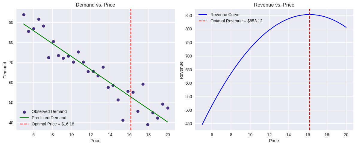
The first plot shows:
- Observed demand (scatter)
- Predicted demand curve (green line)
- Optimal price (red dashed line)
The second plot:
- Revenue curve over price
- Optimal price with corresponding maximum revenue
This helps managers visualize:
- How demand drops as price increases
- Where revenue peaks — the sweet spot
🎯 Conclusion
With just a few lines of Python, we’ve:
- Learned demand behavior from data
- Built a revenue model
- Optimized pricing to maximize profit
This is a basic framework, but in production systems, you could extend this with:
- Time series forecasting (seasonality)
- Price elasticity models
- Multi-product optimization
- Bayesian or probabilistic models
Let data guide your pricing decisions — because guessing is expensive.