In competitive markets, companies often face strategic dilemmas:
- How much to produce?
- How much to spend on advertising?
- How should they respond to a rival’s pricing?
Game theory offers a powerful toolkit for analyzing such questions.
In this post, we’ll look at a simple but insightful example of Cournot competition — a duopoly model — and solve it using Python.
🎯 Problem Overview: Cournot Duopoly
Imagine two firms, Firm A and Firm B, competing by choosing the quantity of output to produce, $q_A$ and $q_B$, respectively.
The price in the market depends on the total quantity produced:
$$
P(Q) = a - bQ \quad \text{where} \quad Q = q_A + q_B
$$
Each firm aims to maximize profit:
$$
\pi_i = q_i \cdot P(Q) - c q_i
$$
Where:
- $a$: maximum price consumers will pay when quantity is 0
- $b$: how price drops with increased quantity
- $c$: marginal cost of production
Each firm’s decision affects the other’s profit, so it’s a strategic setting — perfect for game theory!
🔢 Solving Cournot Equilibrium in Python
Let’s consider:
- $a = 100$
- $b = 1$
- $c = 10$
We’ll solve for the Nash equilibrium: the quantities $q_A^*, q_B^*$ such that neither firm can increase profit by changing its own output unilaterally.
Here’s the code:
1 | import numpy as np |
Nash Equilibrium:
  Firm A: 30.00 units
  Firm B: 30.00 units
🔍 Code Explanation
profit_Aandprofit_Bdefine each firm’s profit as a function of its output and the rival’s output.best_response_Aandbest_response_Bfind the profit-maximizing quantity given the other firm’s output using numerical optimization (scipy.optimize.minimize).find_nash_equilibriumalternates between best responses until the output quantities converge — this gives us the Nash equilibrium.
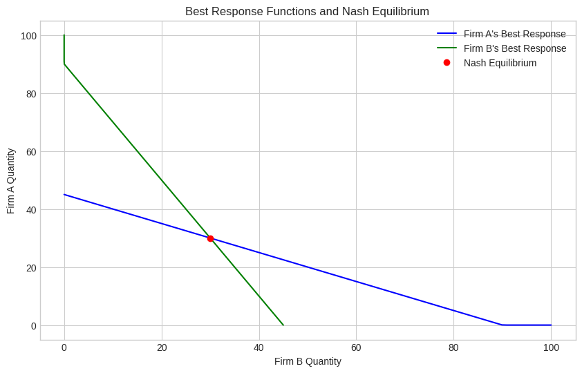
📊 Visualizing Best Response Functions
To better understand the strategic interaction, let’s plot the best response functions:
1 | q_vals = np.linspace(0, 100, 100) |
📈 Graph Explanation
- The blue curve shows Firm A’s best response for every output level of Firm B.
- The green curve shows Firm B’s best response for every output level of Firm A (we flip axes for visualization).
- The red dot is where both best responses intersect — the Nash equilibrium.
This visualization makes it clear: each firm’s output is optimal given the other’s output at the intersection point.
✅ Conclusion
In this blog post, we’ve:
- Modeled a Cournot duopoly using game theory.
- Solved for the Nash equilibrium numerically with Python.
- Visualized strategic interactions with best response curves.
Such models help economists and strategists understand competitive behaviors, predict outcomes, and guide decision-making in real markets.