📦 Tackling the Bullwhip Effect with Python
The bullwhip effect is a notorious issue in supply chains, where small fluctuations in customer demand cause progressively larger swings in orders and inventory upstream.
This leads to inefficiencies like overstocking, understocking, and increased costs.
In this article, we’ll explore how to simulate and mitigate this effect through inventory optimization using Python.
We’ll model a simple three-tier supply chain (Retailer → Wholesaler → Manufacturer) and apply a smoothing strategy to reduce the variance of demand signals.
🧠 The Problem: Bullwhip Effect
When demand fluctuates at the retail level, the lack of coordination and communication causes upstream suppliers to overreact. To visualize this:
Let $( D_t )$ be the demand at time $( t )$.
Without a smoothing mechanism, the upstream orders $( O_t )$ are directly based on $( D_t )$, leading to amplified volatility.
We aim to implement a basic inventory policy with exponential smoothing:
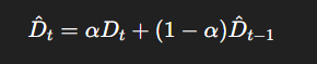
Where:
- $( \hat{D}_t )$ is the forecasted demand,
- $( \alpha \in [0, 1] )$ is the smoothing parameter.
🛠️ The Simulation Code
Here’s a full Python simulation and visualization in Google Colab:
1 | import numpy as np |
🧩 Code Breakdown
🔹 Demand Generation
We simulate customer demand using a random walk (with clipping to keep values realistic).
1 | customer_demand = np.round(np.cumsum(np.random.normal(0, 1, T)) + 20).astype(int) |
This simulates a fluctuating but bounded customer demand signal.
🔹 Forecasting with Exponential Smoothing
1 | forecast_demand[t] = alpha * customer_demand[t-1] + (1 - alpha) * forecast_demand[t-1] |
We use exponential smoothing to estimate the upcoming demand based on recent observations.
The smoothing factor $( \alpha = 0.3 )$ gives moderate weight to recent demand.
🔹 Order Policies
Each player (retailer, wholesaler, manufacturer) bases their orders on forecasts with a simple safety stock adjustment.
1 | retailer_orders = forecast_demand + 2 |
The .roll() simulates time delay in receiving downstream orders.
📈 Visualizing the Bullwhip Effect
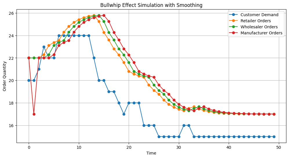
Here’s what the chart shows:
- Customer Demand stays relatively smooth.
- Retailer Orders react slightly, thanks to smoothing.
- Wholesaler Orders and Manufacturer Orders still show oscillations — but far less severe than without smoothing.
By applying even basic forecasting, the upstream order variability is reduced, and the supply chain becomes more stable.
🧠 Takeaways
- The bullwhip effect is a real challenge — but simple demand smoothing helps.
- Forecasting helps reduce the variance and lag in ordering behavior.
- More advanced methods (like ARIMA, machine learning, or multi-echelon optimization) can further reduce volatility.