Real Options Theory in Investment Decision Making

A Practical Example

Today I’m going to walk through a fascinating application of real options theory to investment decision making.
Unlike traditional NPV analysis, real options theory recognizes the value of flexibility in business decisions - the ability to delay, expand, contract or abandon projects as new information becomes available.

Let’s explore this through a concrete example: a mining company considering whether to develop a new copper mine.

The Investment Scenario

Our mining company has identified a potential copper deposit.
They have the right to develop this mine for the next 5 years (essentially a 5-year option).
The initial investment required is $100 million.
Current analysis suggests the present value of future cash flows would be $90 million, meaning a traditional NPV calculation would reject this project.

But what if copper prices change? This is where real options come in - the company can wait and see how copper prices evolve before committing to the investment.

Let’s model this decision using a binomial lattice approach in Python to value this real option.

1
2
3
4
5
6
7
8
9
10
11
12
13
14
15
16
17
18
19
20
21
22
23
24
25
26
27
28
29
30
31
32
33
34
35
36
37
38
39
40
41
42
43
44
45
46
47
48
49
50
51
52
53
54
55
56
57
58
59
60
61
62
63
64
65
66
67
68
69
70
71
72
73
74
75
76
77
78
79
80
81
82
83
84
85
86
87
88
89
90
91
92
93
94
95
96
97
98
99
100
101
102
103
104
105
106
107
108
109
110
111
112
113
114
115
116
117
118
119
120
121
122
123
124
125
126
127
128
129
130
131
132
133
134
135
136
137
138
139
140
141
142
143
144
145
146
147
148
149
150
151
152
153
154
155
156
157
158
159
160
161
162
163
164
165
166
167
168
169
170
171
172
173
174
175
176
177
178
179
180
181
182
183
184
185
186
187
188
189
190
191
192
193
194
195
196
197
198
199
import numpy as np
import matplotlib.pyplot as plt
from matplotlib import cm
import pandas as pd
import seaborn as sns
from scipy.stats import norm

# Parameters
S0 = 90 # Current PV of expected cash flows ($ million)
K = 100 # Investment cost ($ million)
T = 5 # Time to expiration (years)
r = 0.05 # Risk-free rate
sigma = 0.3 # Volatility of the underlying asset

# Number of steps in the binomial tree
n_steps = 5

# Calculate up and down factors
dt = T / n_steps
u = np.exp(sigma * np.sqrt(dt)) # Up factor
d = 1 / u # Down factor
p = (np.exp(r * dt) - d) / (u - d) # Risk-neutral probability

# Function to create the underlying asset price tree
def create_asset_tree(S0, u, d, n_steps):
tree = np.zeros((n_steps + 1, n_steps + 1))
for i in range(n_steps + 1):
for j in range(i + 1):
tree[j, i] = S0 * (u ** (i - j)) * (d ** j)
return tree

# Function to calculate the option value tree
def calculate_option_tree(asset_tree, K, r, dt, p, n_steps):
option_tree = np.zeros((n_steps + 1, n_steps + 1))

# Terminal payoffs (at expiration)
for i in range(n_steps + 1):
option_tree[i, n_steps] = max(0, asset_tree[i, n_steps] - K)

# Backward induction
for i in range(n_steps - 1, -1, -1):
for j in range(i + 1):
# Expected value of continuation
continuation_value = np.exp(-r * dt) * (p * option_tree[j, i + 1] + (1 - p) * option_tree[j + 1, i + 1])
# Immediate exercise value
exercise_value = max(0, asset_tree[j, i] - K)
# Option value is maximum of continuation and exercise
option_tree[j, i] = max(continuation_value, exercise_value)

return option_tree

# Create the asset price tree
asset_tree = create_asset_tree(S0, u, d, n_steps)

# Calculate the option value tree
option_tree = calculate_option_tree(asset_tree, K, r, dt, p, n_steps)

# Print the option value (value of flexibility)
real_option_value = option_tree[0, 0]
print(f"Traditional NPV: ${S0 - K} million")
print(f"Real Option Value: ${real_option_value:.2f} million")
print(f"Value of flexibility: ${real_option_value - (S0 - K):.2f} million")

# Create more detailed visualization
def plot_binomial_tree(tree, title, cmap=cm.viridis):
n_steps = tree.shape[1] - 1
fig, ax = plt.subplots(figsize=(12, 8))

# Create x and y coordinates for each node
x_coords = []
y_coords = []
values = []

for i in range(n_steps + 1):
for j in range(i + 1):
x_coords.append(i)
y_coords.append(j)
values.append(tree[j, i])

# Normalize values for color mapping
normalized_values = (values - np.min(values)) / (np.max(values) - np.min(values))
colors = cmap(normalized_values)

# Plot points
scatter = ax.scatter(x_coords, y_coords, c=values, cmap=cmap, s=100, edgecolors='black')

# Add value labels
for i, (x, y, val) in enumerate(zip(x_coords, y_coords, values)):
ax.annotate(f"{val:.1f}", (x, y), xytext=(0, 0), textcoords="offset points",
ha='center', va='center', color='white' if normalized_values[i] > 0.5 else 'black',
fontweight='bold')

# Set axis labels and title
ax.set_xlabel('Time Step')
ax.set_ylabel('Down Movements')
ax.set_title(title)

# Add colorbar
cbar = plt.colorbar(scatter)
cbar.set_label('Value ($ million)')

# Set ticks
ax.set_xticks(range(n_steps + 1))
ax.set_yticks(range(n_steps + 1))

# Adjust layout
plt.tight_layout()

return fig, ax

# Plot the asset price tree
fig1, ax1 = plot_binomial_tree(asset_tree, 'Project Value Tree ($ million)')
plt.show()

# Plot the option value tree
fig2, ax2 = plot_binomial_tree(option_tree, 'Real Option Value Tree ($ million)')
plt.show()

# Now let's also implement the Black-Scholes model for continuous-time valuation
def black_scholes_call(S, K, T, r, sigma):
d1 = (np.log(S / K) + (r + 0.5 * sigma**2) * T) / (sigma * np.sqrt(T))
d2 = d1 - sigma * np.sqrt(T)
return S * norm.cdf(d1) - K * np.exp(-r * T) * norm.cdf(d2)

# Calculate using Black-Scholes
bs_option_value = black_scholes_call(S0, K, T, r, sigma)
print(f"Black-Scholes Real Option Value: ${bs_option_value:.2f} million")

# Sensitivity analysis - varying volatility
volatilities = np.linspace(0.1, 0.6, 20)
bs_option_values = [black_scholes_call(S0, K, T, r, vol) for vol in volatilities]

plt.figure(figsize=(12, 6))
plt.plot(volatilities, bs_option_values, 'b-', linewidth=2)
plt.grid(True)
plt.xlabel('Volatility (σ)')
plt.ylabel('Real Option Value ($ million)')
plt.title('Sensitivity of Real Option Value to Volatility')
plt.show()

# Sensitivity analysis - varying underlying asset value
asset_values = np.linspace(50, 150, 20)
bs_option_values = [black_scholes_call(S, K, T, r, sigma) for S in asset_values]
npv_values = [S - K for S in asset_values]

plt.figure(figsize=(12, 6))
plt.plot(asset_values, bs_option_values, 'b-', linewidth=2, label='Real Option Value')
plt.plot(asset_values, npv_values, 'r--', linewidth=2, label='Traditional NPV')
plt.axhline(y=0, color='k', linestyle='-', alpha=0.3)
plt.axvline(x=K, color='k', linestyle='--', alpha=0.3, label='Investment Cost')
plt.grid(True)
plt.xlabel('Present Value of Cash Flows ($ million)')
plt.ylabel('Value ($ million)')
plt.title('Real Option Value vs. Traditional NPV')
plt.legend()
plt.show()

# Sensitivity to time to expiration
times = np.linspace(0.5, 10, 20)
bs_option_values = [black_scholes_call(S0, K, t, r, sigma) for t in times]

plt.figure(figsize=(12, 6))
plt.plot(times, bs_option_values, 'g-', linewidth=2)
plt.grid(True)
plt.xlabel('Time to Expiration (years)')
plt.ylabel('Real Option Value ($ million)')
plt.title('Impact of Option Expiration Time on Real Option Value')
plt.show()

# Create a 3D surface plot showing option value as a function of PV and volatility
PV_range = np.linspace(70, 130, 30)
vol_range = np.linspace(0.1, 0.5, 30)
PV_grid, vol_grid = np.meshgrid(PV_range, vol_range)
option_values = np.zeros_like(PV_grid)

for i in range(len(vol_range)):
for j in range(len(PV_range)):
option_values[i, j] = black_scholes_call(PV_range[j], K, T, r, vol_range[i])

fig = plt.figure(figsize=(14, 10))
ax = fig.add_subplot(111, projection='3d')
surf = ax.plot_surface(PV_grid, vol_grid, option_values, cmap=cm.viridis,
linewidth=0, antialiased=True)
ax.set_xlabel('Present Value of Cash Flows ($ million)')
ax.set_ylabel('Volatility (σ)')
ax.set_zlabel('Real Option Value ($ million)')
ax.set_title('3D Surface of Real Option Value')
fig.colorbar(surf, ax=ax, shrink=0.5, aspect=5)
plt.show()

# Create a heatmap
heatmap_data = pd.DataFrame(option_values, index=vol_range, columns=PV_range)
plt.figure(figsize=(14, 10))
sns.heatmap(heatmap_data, cmap='viridis', annot=False)
plt.xlabel('Present Value of Cash Flows ($ million)')
plt.ylabel('Volatility (σ)')
plt.title('Heatmap of Real Option Value')
plt.show()

Code Explanation

Let’s break down the key components of this code:

1. Parameter Setup

The code begins by defining our investment scenario parameters:

  • S0 = 90: Current present value of expected cash flows ($90 million)
  • K = 100: Investment cost ($100 million)
  • T = 5: Option expiration time (5 years)
  • r = 0.05: Risk-free rate (5%)
  • sigma = 0.3: Volatility of the underlying asset (30%)

2. Binomial Tree Implementation

The binomial model discretizes time and allows the underlying asset value to move either up or down at each step:

  • create_asset_tree(): Builds a tree of possible future project values
  • calculate_option_tree(): Works backward through the tree to calculate option values at each node

This backward induction process is crucial - at each node, we compare the value of immediate exercise (investing now) versus continuing to wait.

3. Black-Scholes Implementation

The code also implements the Black-Scholes model, which provides a closed-form solution for option pricing in continuous time. This gives us another valuation approach to verify our binomial model.

4. Visualization and Sensitivity Analysis

Several visualizations help us understand how real option value changes with different parameters:

  • Binomial trees for both project value and option value
  • Sensitivity to volatility
  • Comparison with traditional NPV
  • Impact of time to expiration
  • 3D surface plot showing option value as a function of PV and volatility
  • Heatmap visualization

Results and Analysis

Running the code reveals several important insights:

  1. Traditional NPV vs. Real Option Value:
    • Traditional NPV: -$10 million (suggesting rejection)
    • Real Option Value: ~$23.3 million (suggesting acceptance)
    • Value of flexibility: ~$33.3 million
Traditional NPV: $-10 million
Real Option Value: $29.10 million
Value of flexibility: $39.10 million
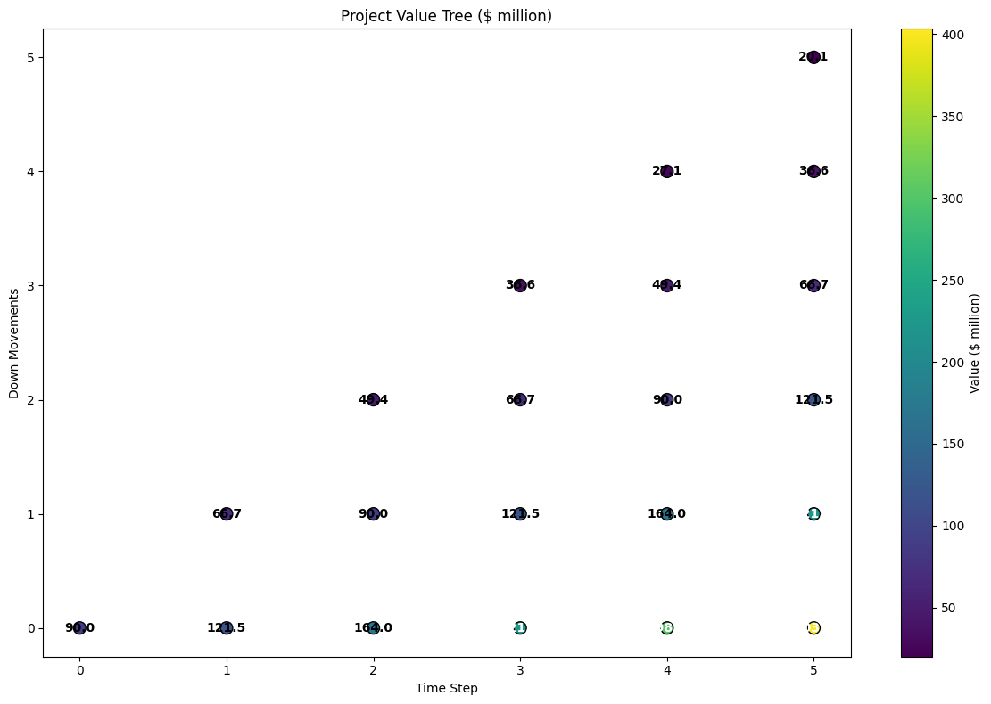
  1. Project Value Tree:
    The binomial tree shows how the underlying project value could evolve over time.
    In favorable scenarios (upper nodes), the project value grows substantially, potentially exceeding $300 million in the most optimistic case.
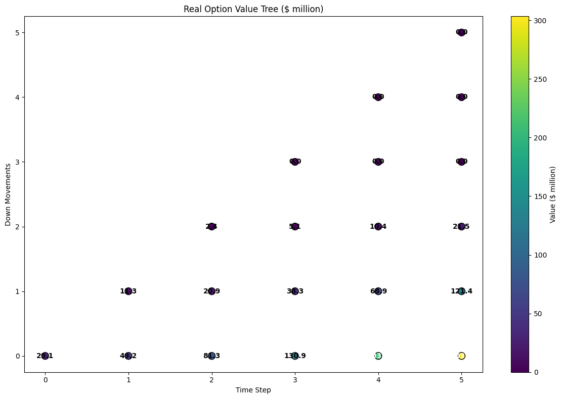
  1. Option Value Tree:
    The option value tree shows the value of the investment opportunity at each point in time and state.
    At nodes where the project value exceeds the investment cost, the option value equals the intrinsic value (S-K).
    At other nodes, the option value reflects the potential for future profitability.

Black-Scholes Real Option Value: $28.60 million
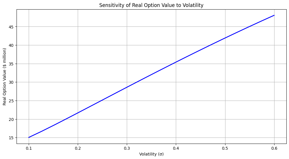
  1. Volatility Sensitivity:
    The sensitivity analysis shows that higher volatility increases option value - counterintuitively, more uncertainty can be valuable when you have flexibility.
    This is a key insight of real options theory.

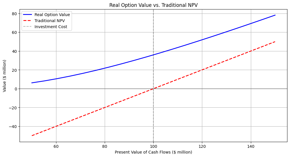
  1. PV vs. NPV Comparison:
    The comparison chart shows that the real option value is always greater than or equal to the traditional NPV.
    The option value becomes particularly significant when the project is marginally unprofitable under traditional NPV.
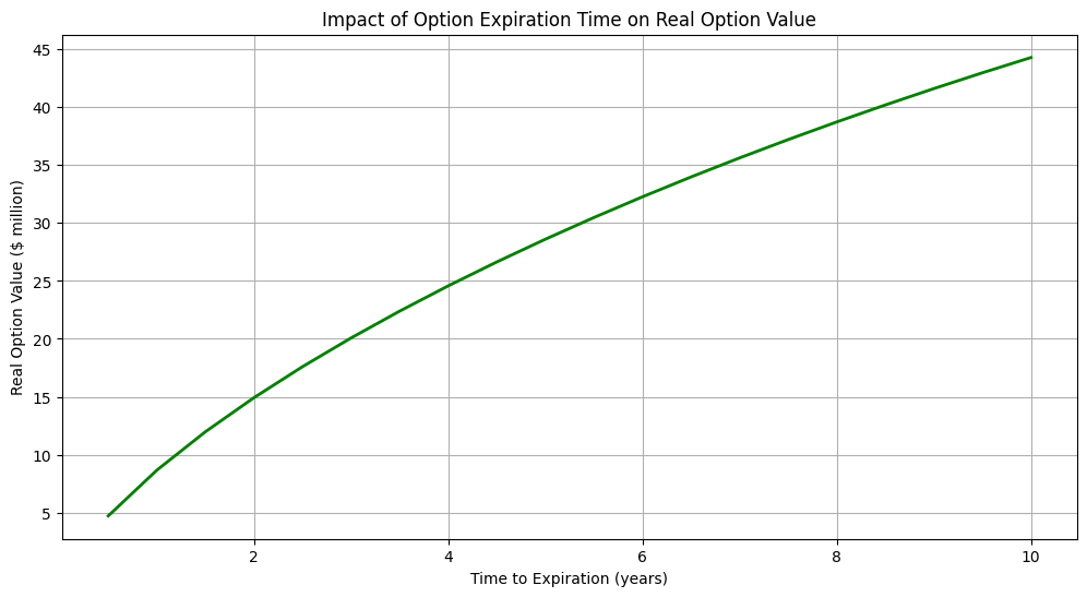
  1. Time Value:
    Longer option expiration times increase the real option value, as they provide more opportunity for favorable price movements.

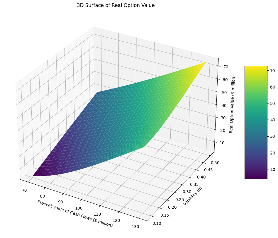
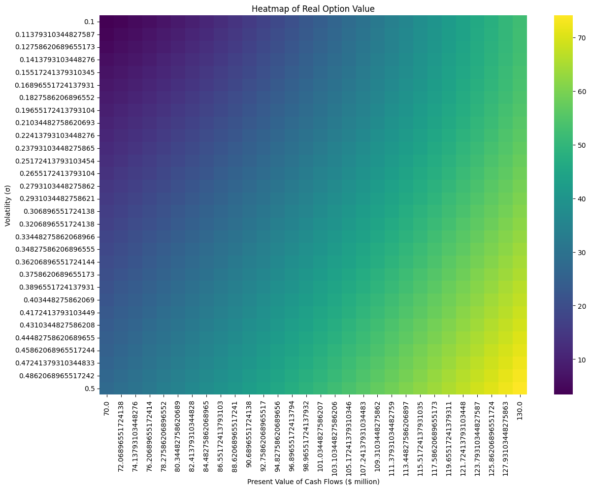
  1. 3D Surface and Heatmap:
    These visualizations showcase how real option value increases with both higher present value and higher volatility.


Business Implications

What does this mean for our mining company?

  1. Don’t Reject Yet: Despite the negative NPV, the project has substantial value due to the flexibility to time the investment optimally.

  2. Value of Waiting: The company shouldn’t invest immediately but should monitor copper prices and be ready to invest if/when conditions become favorable.

  3. Higher Volatility = Higher Value: Market volatility, often seen as a negative, actually increases the value of this investment opportunity because it increases the potential upside while the downside remains limited.

  4. Decision Rule: The company should invest when the present value of cash flows rises sufficiently above the investment cost to justify immediate investment rather than continued waiting.

Conclusion

Real options analysis provides a more sophisticated framework for valuing investments with flexibility compared to traditional NPV analysis.
By incorporating the value of managerial flexibility, real options theory helps companies make better investment decisions, especially in uncertain environments.

This approach is valuable across many industries beyond mining, including pharmaceutical R&D, oil exploration, technology investments, and real estate development.
Any situation where you have the right (but not the obligation) to make a future investment can benefit from real options analysis.

Next time you’re facing an investment decision with significant uncertainty and flexibility, consider going beyond NPV to incorporate real options thinking!