A Practical Implementation
In today’s increasingly interconnected world, multi-agent systems are becoming more prevalent in various domains from economics to computer networks.
One of the most fascinating challenges in these systems is how to optimally allocate limited resources among competing agents.
Let’s dive into a concrete example and solve it step by step using Python.
The Problem: Task Allocation in a Team of Robots
Imagine we have a team of robots (our agents) that need to complete various tasks in a warehouse.
Each robot has different capabilities and efficiencies for different tasks, and we need to allocate the tasks optimally to maximize overall efficiency.
This is a classic resource allocation problem in multi-agent systems.
We’ll model this as a linear optimization problem and solve it using Python’s powerful optimization libraries.
Let’s implement this solution:
1 | import numpy as np |
Understanding the Code: A Deep Dive
Let’s break down the two approaches I’ve implemented for resource allocation in multi-agent systems:
Example 1: Simple Task Allocation with Hungarian Algorithm
The first example demonstrates a classic one-to-one matching problem where each robot can be assigned to exactly one task to maximize overall efficiency.
This is perfectly suited for the Hungarian algorithm (implemented in Python as linear_sum_assignment).
The key components of this implementation are:
Efficiency Matrix: We create a matrix where each cell represents how efficiently a particular robot can perform a specific task.
Higher values indicate better performance.Cost Matrix Conversion: Since the Hungarian algorithm minimizes cost, we negate the efficiency values to convert the maximization problem into a minimization one.
Optimal Assignment: The algorithm returns the row and column indices that give us the optimal assignment.
The mathematical formulation of this problem can be represented as:
$$\max \sum_{i=1}^{n} \sum_{j=1}^{m} e_{ij} \cdot x_{ij}$$
Subject to:
$$\sum_{j=1}^{m} x_{ij} = 1 \quad \forall i$$
$$\sum_{i=1}^{n} x_{ij} = 1 \quad \forall j$$
$$x_{ij} \in {0, 1} \quad \forall i,j$$
Where:
- $e_{ij}$ is the efficiency of robot $i$ performing task $j$
- $x_{ij}$ is a binary variable that equals 1 if robot $i$ is assigned to task $j$, and 0 otherwise
Example 2: Resource-Constrained Allocation with Linear Programming
The second example tackles a more complex scenario where tasks require various resources, and robots have limited resource capacities.
This requires linear programming to solve (using PuLP library).
Key components include:
Multiple Resources: Each task requires different amounts of multiple resource types.
Resource Constraints: Each robot has limited capacity for each resource type.
Binary Variables: We use binary variables to represent whether a robot is assigned to a task.
The mathematical formulation can be expressed as:
$$\max \sum_{i=1}^{n} \sum_{j=1}^{m} e_{ij} \cdot x_{ij}$$
Subject to:
$$\sum_{i=1}^{n} x_{ij} \leq 1 \quad \forall j$$
$$\sum_{j=1}^{m} r_{jk} \cdot x_{ij} \leq c_{ik} \quad \forall i, k$$
$$x_{ij} \in {0, 1} \quad \forall i,j$$
Where:
- $e_{ij}$ is the efficiency of robot $i$ performing task $j$
- $x_{ij}$ is a binary variable that equals 1 if robot $i$ is assigned to task $j$
- $r_{jk}$ is the amount of resource $k$ required for task $j$
- $c_{ik}$ is the capacity of resource $k$ available to robot $i$
Visualizing the Results
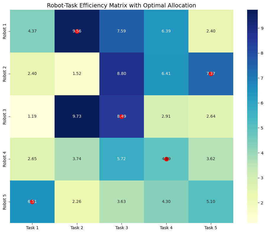
For the first example, we created a heatmap of the efficiency matrix with red circles highlighting the optimal assignments.
This makes it easy to see which robot is matched with which task.
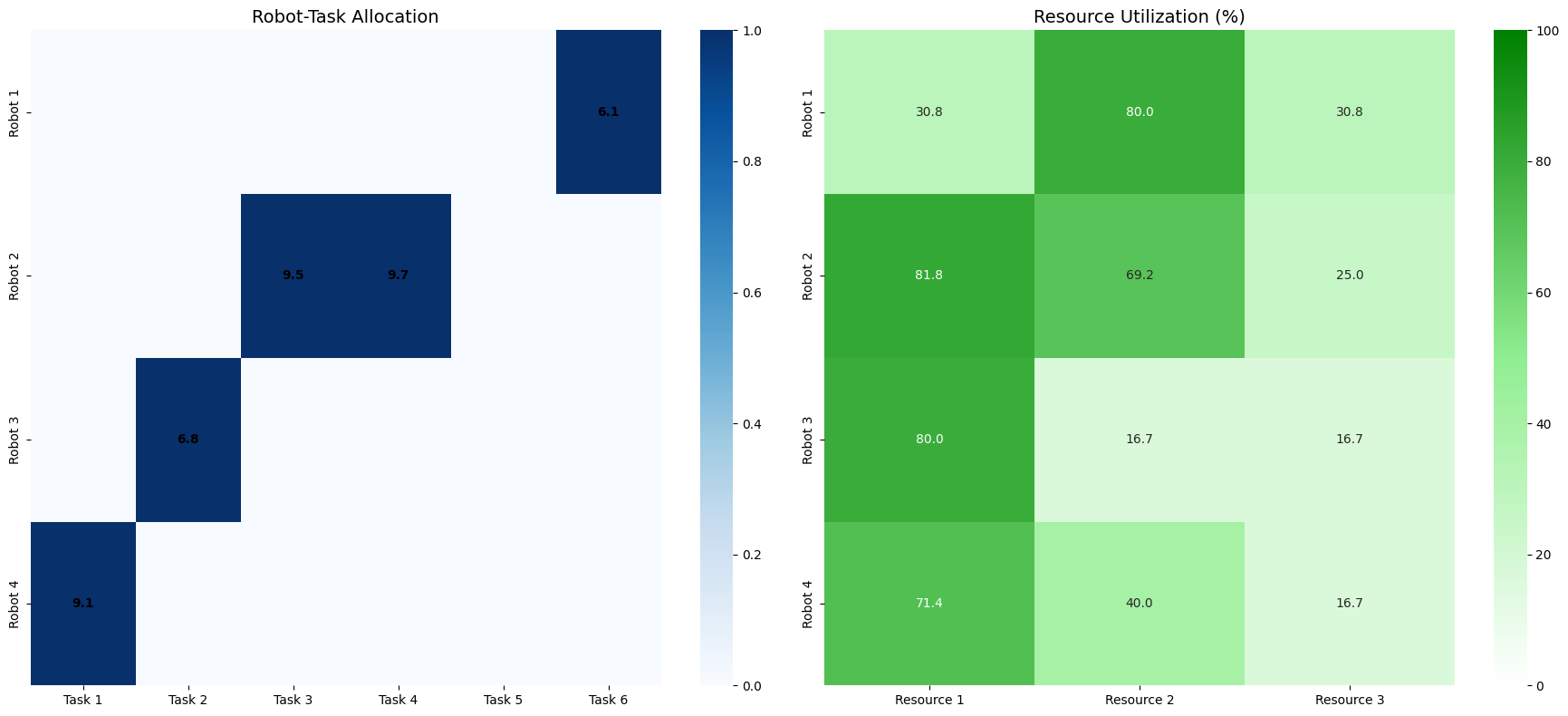
For the resource-constrained example, we created multiple visualizations:
- Allocation Matrix: Shows which robot is assigned to which task along with the efficiency values.
Example 1: Simple Task Allocation Using Hungarian Algorithm
============================================================
Efficiency Matrix (Robot vs Task):
           Task 1    Task 2    Task 3    Task 4    Task 5
Robot 1  4.370861  9.556429  7.587945  6.387926  2.404168
Robot 2  2.403951  1.522753  8.795585  6.410035  7.372653
Robot 3  1.185260  9.729189  8.491984  2.911052  2.636425
Robot 4  2.650641  3.738180  5.722808  4.887505  3.621062
Robot 5  6.506676  2.255445  3.629302  4.297257  5.104630

Optimal Allocation:
Assign Robot 1 to Task 2 (Efficiency: 9.56)
Assign Robot 2 to Task 5 (Efficiency: 7.37)
Assign Robot 3 to Task 3 (Efficiency: 8.49)
Assign Robot 4 to Task 4 (Efficiency: 4.89)
Assign Robot 5 to Task 1 (Efficiency: 6.51)

Total Efficiency: 36.82
- Resource Utilization: Shows how much of each robot’s resource capacity is being used (as a percentage).
Example 2: Resource Constrained Allocation Using Linear Programming
============================================================
Task Efficiency Matrix (Robot vs Task):
Task 1 Task 2 Task 3 Task 4 Task 5 Task 6
Robot 1 7.851760 1.996738 5.142344 5.924146 0.464504 6.075449
Robot 2 1.705241 0.650516 9.488855 9.656320 8.083973 3.046138
Robot 3 0.976721 6.842330 4.401525 1.220382 4.951769 0.343885
Robot 4 9.093204 2.587800 6.625223 3.117111 5.200680 5.467103
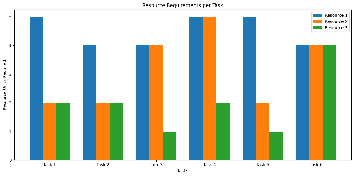
Resource Requirements for Each Task:
Resource 1 Resource 2 Resource 3
Task 1 5 2 2
Task 2 4 2 2
Task 3 4 4 1
Task 4 5 5 2
Task 5 5 2 1
Task 6 4 4 4
Resource Capacities for Each Robot:
Resource 1 Resource 2 Resource 3
Robot 1 13 5 13
Robot 2 11 13 12
Robot 3 5 12 12
Robot 4 7 5 12
Status: Optimal
Optimal Allocation:
Assign Robot 1 to Task 6 (Efficiency: 6.08)
Assign Robot 2 to Task 3 (Efficiency: 9.49)
Assign Robot 2 to Task 4 (Efficiency: 9.66)
Assign Robot 3 to Task 2 (Efficiency: 6.84)
Assign Robot 4 to Task 1 (Efficiency: 9.09)
Total Efficiency: 41.16
Resource Usage for Each Robot:
Resource 1 Resource 2 Resource 3
Robot 1 4.0 4.0 4.0
Robot 2 9.0 9.0 3.0
Robot 3 4.0 2.0 2.0
Robot 4 5.0 2.0 2.0
Resource Utilization (%):
Resource 1 Resource 2 Resource 3
Robot 1 30.769231 80.000000 30.769231
Robot 2 81.818182 69.230769 25.000000
Robot 3 80.000000 16.666667 16.666667
Robot 4 71.428571 40.000000 16.666667
- Task Resource Requirements: A bar chart showing how much of each resource is required by each task.
These visualizations help us understand the trade-offs and constraints in multi-agent resource allocation problems.
Practical Applications
This type of optimization is applicable in many real-world scenarios:
- Cloud computing resource allocation
- Supply chain management
- Emergency service dispatch
- Factory production planning
- Network bandwidth allocation
By optimizing resource allocation, we can significantly improve efficiency and reduce costs in multi-agent systems.
Conclusion
Resource allocation in multi-agent systems represents a fascinating intersection of operations research and distributed computing.
The approaches demonstrated here—Hungarian algorithm for simple matching and linear programming for constrained optimization—provide powerful tools for solving these problems.
The key takeaway is that with the right mathematical formulation and optimization techniques, we can find efficient solutions to complex resource allocation problems, even with multiple constraints and objectives.