Let’s consider a basic aerodynamics problem: Calculating the Drag Force on an Object Moving Through Air.
Problem Description
The drag force $( F_d )$ experienced by an object moving through a fluid (like air) can be calculated using the drag equation:
$$
F_d = \frac{1}{2} C_d \rho A v^2
$$
- $ F_d $ = Drag Force (in $Newtons$)
- $ C_d $ = Drag Coefficient (depends on the shape of the object, e.g., $0.47$ for a sphere)
- $ \rho $ = Air Density (in $ kg/m^3 $, typically $1.225$ $ kg/m^3 $ at sea level)
- $ A $ = Cross-sectional Area of the object (in $ m^2 $)
- $ v $ = Velocity of the object relative to the air (in $ m/s $)
Scenario
Let’s calculate how the drag force changes with velocity for a spherical object (like a ball) with:
- Radius: $0.1$ $m$ (cross-sectional area $ A = \pi r^2 $)
- Drag Coefficient $ C_d $: $0.47$ (typical for a sphere)
- Air Density $ \rho $: $1.225$ $ kg/m^3 $
We will plot the drag force for velocities ranging from $0$ to $100$ $m/s$.
Python Implementation
1 | import numpy as np |
Explanation of the Code
Constants:
Cd = 0.47: Drag coefficient for a sphere.rho = 1.225: Air density at sea level.radius = 0.1: Radius of the sphere.A = np.pi * radius**2: Cross-sectional area calculated using $ A = \pi r^2 $.
Velocity Range:
np.linspace(0, 100, 200): Generates $200$ evenly spaced velocity points from $0$ to $100$ $m/s$.
Drag Force Calculation:
F_d = 0.5 * Cd * rho * A * velocities**2: Computes the drag force for each velocity.
Plotting:
- The graph plots Velocity (m/s) on the x-axis and Drag Force (N) on the y-axis.
Interpreting the Graph
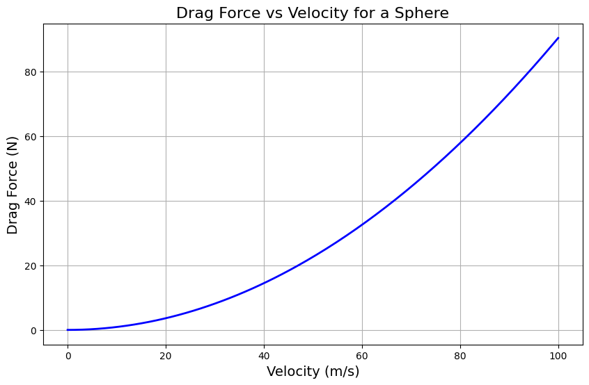
- Shape of the Curve: The drag force increases quadratically with velocity, as indicated by the $ v^2 $ term in the equation.
- At Low Speeds: Drag force is minimal, nearly $zero$ at low velocities.
- At High Speeds: The drag force increases significantly, demonstrating why aerodynamics becomes crucial in high-speed applications like racing or aerospace engineering.