Shannon Entropy of a Discrete Probability Distribution

Problem Description

In information theory, Shannon entropy quantifies the amount of uncertainty in a probability distribution.

It is given by the formula:

H(X)=−n∑i=1P(xi)log2P(xi)

• P(xi) is the probability of the i-th event.
• H(X) is the entropy in bits.

We will:

1. Calculate the Shannon entropy of a discrete probability distribution.
2. Visualize how entropy changes with different probability distributions.

---

Python Solution

import numpy as np
import matplotlib.pyplot as plt

def shannon_entropy(probabilities):
    """
    Calculate the Shannon entropy of a discrete probability distribution.

    Parameters:
        probabilities: List or array of probabilities (must sum to 1).

    Returns:
        entropy: Shannon entropy in bits.
    """
    probabilities = np.array(probabilities)
    # Ensure probabilities are valid
    assert np.isclose(np.sum(probabilities), 1), "Probabilities must sum to 1."
    assert np.all(probabilities >= 0), "Probabilities cannot be negative."

    # Calculate entropy
    entropy = -np.sum(probabilities * np.log2(probabilities + 1e-10))  # Add small value to avoid log(0)
    return entropy

# Define example probability distributions
distributions = {
    "Uniform": [0.25, 0.25, 0.25, 0.25],
    "Biased": [0.7, 0.1, 0.1, 0.1],
    "Highly Skewed": [0.95, 0.05],
    "Equal Binary": [0.5, 0.5],
}

# Calculate entropy for each distribution
entropies = {name: shannon_entropy(dist) for name, dist in distributions.items()}

# Display results
for name, entropy in entropies.items():
    print(f"Entropy of {name} distribution: {entropy:.4f} bits")

# Visualization
fig, ax = plt.subplots(figsize=(10, 6))

# Plot each distribution
for name, dist in distributions.items():
    x = range(len(dist))
    ax.bar(x, dist, alpha=0.7, label=f"{name} (H={entropies[name]:.2f})")
    for i, prob in enumerate(dist):
        ax.text(i, prob + 0.02, f"{prob:.2f}", ha='center', fontsize=10)

# Add labels, legend, and title
ax.set_title("Discrete Probability Distributions and Their Entropy", fontsize=16)
ax.set_xlabel("Events", fontsize=12)
ax.set_ylabel("Probability", fontsize=12)
ax.set_ylim(0, 1.1)
ax.legend()
plt.show()

---

Explanation of the Code

1. Shannon Entropy Calculation:

   • The function shannon_entropy() takes a list of probabilities as input.
   • It ensures the input is valid (probabilities sum to 1 and are non-negative).
   • The entropy formula is implemented using (−∑P(x)log2P(x)), with a small offset (1e−10) to handle probabilities of zero.

2. Example Distributions:

   • Uniform: All events are equally likely ([0.25,0.25,0.25,0.25]).
   • Biased: One event dominates ([0.7,0.1,0.1,0.1]).
   • Highly Skewed: One event is almost certain ([0.95,0.05]).
   • Equal Binary: Two equally likely events ([0.5,0.5]).

3. Visualization:

   • Each distribution is plotted as a bar chart, with labels showing the probabilities and their corresponding entropies.

---

Results

Entropy Values:

Entropy of Uniform distribution: 2.0000 bits
Entropy of Biased distribution: 1.3568 bits
Entropy of Highly Skewed distribution: 0.2864 bits
Entropy of Equal Binary distribution: 1.0000 bits

• Uniform Distribution: (H=2.0,bits) (Maximum entropy for 4 events).
• Biased Distribution: (H=1.3568,bits).
• Highly Skewed Distribution: (H=0.2864,bits) (Almost no uncertainty).
• Equal Binary Distribution: (H=1.0,bits).

Graph:

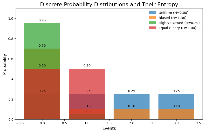
• The bar chart shows the probability distributions for each example.
• Entropy values are displayed in the legend.

---

Insights

1. Uniform Distribution:

   • Maximizes entropy since all events are equally likely.
   • Maximum uncertainty about the outcome.

2. Biased and Highly Skewed Distributions:

   • Lower entropy as probabilities become more uneven.
   • Greater certainty about likely outcomes.

3. Equal Binary Distribution:

   • Entropy is 1 bit, which aligns with the classic case of a fair coin toss.

---

Conclusion

This example illustrates how entropy quantifies uncertainty in probability distributions.

It provides insights into how information theory applies to real-world problems like communication systems, cryptography, and data compression.

The Python implementation and visualization make these concepts clear and accessible.