Example: Modeling Population Growth with Logistic Growth Equation
In Environmental Mathematics, one of the fundamental models used to describe the growth of populations, such as animal populations or human populations, is the Logistic Growth Model.
This model accounts for the carrying capacity of the environment, which limits indefinite exponential growth.
Logistic Growth Equation
The Logistic Growth Model is represented by the following differential equation:
$$
\frac{dP}{dt} = rP \left(1 - \frac{P}{K}\right)
$$
- $( P(t) )$ = Population size at time $( t )$
- $( r )$ = Intrinsic growth rate (how quickly the population grows)
- $( K )$ = Carrying capacity (maximum population size that the environment can support)
- $( t )$ = Time
- $( P(0) )$ = Initial population size at $( t = 0 )$
The solution to this equation models the population growth over time and shows an S-shaped curve, where the population grows exponentially when small, then slows down as it approaches the carrying capacity $( K )$.
Problem
- We will use the Logistic Growth Model to model the population growth of a species over time.
- We will visualize how the population changes as a function of time.
- We will explore the effect of different intrinsic growth rates and carrying capacities on the population size.
Steps
- Define the logistic growth equation and its solution.
- Simulate the population growth using $Python$.
- Plot the population size over time for different parameters.
Python Code
1 | import numpy as np |
Explanation of the Code
Logistic Growth Function:
- The function
logistic_growth(t, P0, r, K)computes the population at time $( t )$ using the logistic growth equation.
It takes:t: Time (which can be an array for continuous simulation)P0: The initial population size at time $( t = 0 )$r: The intrinsic growth rate of the populationK: The carrying capacity (maximum population the environment can support)
- The function calculates the population at time $( t )$ using the formula for logistic growth.
- The function
Parameters:
- $( P_0 = 10 )$: Initial population size.
- $( r = 0.5 )$: Intrinsic growth rate (the speed of population growth).
- $( K = 1000 )$: Carrying capacity (the environment can support up to $1000$ individuals).
t = np.linspace(0, 20, 200): We simulate the population over $20$ time units, with $200$ points to generate a smooth curve.
Plotting the Results:
- The first plot visualizes the population growth over time using the logistic model.
- The second plot shows how different intrinsic growth rates (
r = 0.1, 0.3, 0.5, 0.7) affect the population growth.
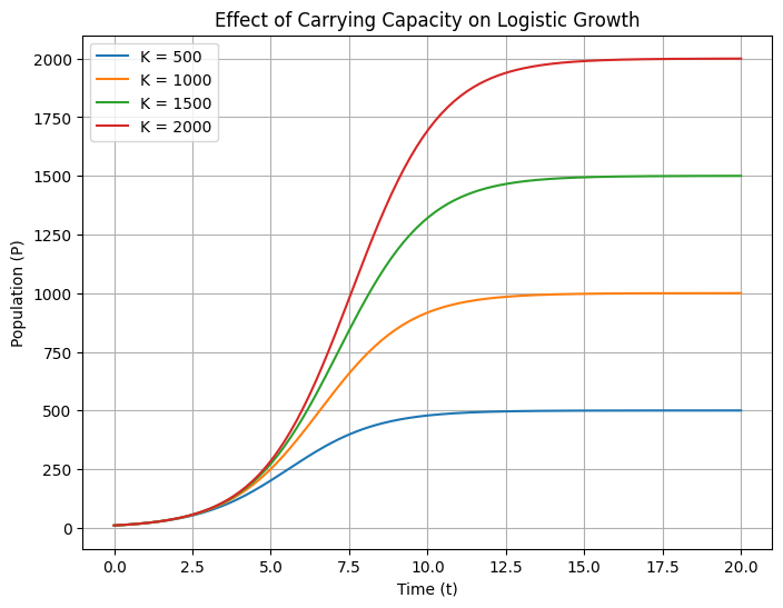
A higher growth rate results in faster population growth. - The third plot shows how varying the carrying capacity (
K = 500, 1000, 1500, 2000) influences the population.
A higher carrying capacity allows the population to grow to a higher final size.
Expected Outcome
Logistic Growth Curve:
The first plot will show the characteristic S-shaped curve.
The population starts growing exponentially, but as it approaches the carrying capacity $( K )$, it slows down and levels off.Effect of Intrinsic Growth Rate:
In the second plot, as the intrinsic growth rate $( r )$ increases, the population grows faster at the beginning, but the population ultimately approaches the same carrying capacity in each case.
The time it takes to reach near the carrying capacity is shorter for higher growth rates.Effect of Carrying Capacity:
In the third plot, increasing the carrying capacity $( K )$ leads to a higher maximum population.
However, the growth curve still follows the same logistic pattern, only the “$ceiling$” is higher.

Result Analysis
The S-shaped curve is a key feature of the logistic growth model, showing how the population grows rapidly at first, but as resources become limited, the growth slows and eventually stabilizes near the carrying capacity.
The intrinsic growth rate $( r )$ affects the speed of growth.
A higher growth rate leads to a quicker approach to the carrying capacity.The carrying capacity $( K )$ defines the maximum population that the environment can support.
If $( K )$ is increased, the population can grow to a higher value before stabilizing.
Conclusion
This example demonstrates how Environmental Mathematics uses mathematical models like logistic growth to understand population dynamics in a given environment.
By adjusting parameters such as the intrinsic growth rate and carrying capacity, we can predict how populations will evolve over time and make informed decisions for environmental management, conservation, and resource allocation.